Decision Trees: A Simple Guide to Making Predictions with Data
Introduction: Making Choices Like a Flowchart
Imagine you are playing a game where you need to guess an animal. You might start by asking questions like: “Does it have fur?”. Based on the answer, you might ask another question, such as “Does it live in the water?”. You keep asking questions, making decisions, until you reach an answer. This step-by-step way of making decisions is how a Decision Tree works in machine learning.
A Decision Tree is a popular type of machine learning algorithm that helps us make predictions or decisions by creating a tree-like structure. It’s a supervised learning algorithm, meaning it learns from data that has already been labeled.
Decision trees are used for two main tasks:
- Classification: Sorting data into different groups or categories. For example, predicting if an email is spam or not spam, or classifying different types of flowers.
- Regression: Predicting a continuous value or number. For example, predicting the price of a house or the temperature tomorrow.
Real-World Examples:
- Medical Diagnosis: Doctors use a similar process when diagnosing an illness. They ask about symptoms (“Do you have a fever?”, “Do you have a cough?”) and make decisions about the cause. In fact, decision tree algorithms are also used to help doctors make these diagnoses more effectively by analyzing large sets of medical data and giving an accurate diagnosis.
- Loan Approval: Banks use decision trees to decide whether to approve a loan. They look at factors like income, credit score, and previous loan history. By using a decision tree model, banks can make informed decisions to approve or reject a loan.
- Customer Churn Prediction: Mobile companies use decision trees to figure out which customers are likely to switch to another provider. They consider things like data usage, calling habits, and customer service interactions. This enables companies to contact those specific customers before they decide to switch, or provide some discounts to keep them with the same company.
- Fraud Detection: Banks and other financial institutions can use a decision tree algorithm to detect fraudulent transactions based on different features such as time of transaction, location of transaction etc.
The Mathematics Behind Decision Trees: Splitting the Data
Decision trees use math to decide how to split the data into different branches.
Entropy and Information Gain
At the core of building a decision tree is the concept of information gain, which is based on a measure called entropy. Think of entropy as the “messiness” or “disorder” in the data. If all the items are of the same type, there is no messiness and the entropy is zero. But when the items are mixed up, we have high entropy.
Here is how we calculate entropy:
The formula for Entropy, \(E(S)\), is given by:
\(E(S) = -\sum_{i=1}^{c} p_i \log_2 p_i\) where:
- E(S): Entropy of the set S
- pi: The proportion of data points in set S that belong to category “i”. For instance, if we have 10 cats and 10 dogs, the proportion of cats is 0.5.
- log2: The logarithm with base 2. This is how to calculate it: If \(log_2 8 = y\) then \({2}^{y} = 8\). Here, \(y = 3\) , because \(2^3 = 8\).
Let’s make it simple with an example. Imagine you have a bag of 10 balls, and 5 are red and 5 are blue.
- Calculate the proportion of each category: Proportion of red balls (p1) = 5/10 = 0.5, and Proportion of blue balls (p2) = 5/10 = 0.5
- Calculate the term for red balls = 0.5 * log2(0.5) = 0.5 * -1 = -0.5
- Calculate the term for blue balls = 0.5 * log2(0.5) = 0.5 * -1 = -0.5
- Entropy, H(S) = -(-0.5 + -0.5) = 1.
If there are all red balls, then it will be 0.
Information Gain (IG) tells you how much a particular question (like “Is it raining?”) helps reduce uncertainty in our data.
-
Measure the reduction in Entropy before and after a split on a subset S using the attribute A.
\[IG(S,A) = E(S) - \sum_{v \in Values(A)} \frac{|S_v|}{|S|} * E(S_v)\]Where:
IG(S, A)is the information gain of splitting the dataset S using feature A.E(S)is the entropy of the original data set.Values(A)represents all possible values for the attribute A.S_vis a subset of S, where all data points have the same valuevfor attribute A.|S_v|is the number of samples in subset S_v.|S|is the number of samples in the original dataset S.E(S_v)is the entropy of the subset S_v.
- The more the IG the better then!
- IG can help the Decision tree grow smarter!
- A split in the decision tree is created when the information gain of the split is maximized.
Prerequisites and Setup
Before you build a decision tree, here are some things you need:
- Data: You need data where you know both the inputs (features) and the answer (target). This is called “labeled data.”
- Basic Math: Familiarity with basic math concepts like percentages and logarithms can help you grasp the formulas, but it’s not essential to use the decision trees.
- Python Libraries:
scikit-learn: The most common library for building machine learning models in Python.pandas: Makes it easy to work with tabular data (like spreadsheets).numpy: Helps with math functions.matplotliborseaborn: For visualizing data (optional).
To install these, open your terminal or command prompt and run:
pip install scikit-learn pandas numpy matplotlib
Tweakable Parameters and Hyperparameters
Decision Trees have many parameters you can adjust to control how they learn. These are also known as hyperparameters. Here are some key ones:
-
max_depth: This controls how deep or tall the tree can get.
-
Effect: A small max_depth makes a simple tree, which may not capture all the complexity in the data (underfitting). But it will be very general. A large max_depth can make the tree too specific to the training data and perform badly on new data (overfitting).
-
Example: max_depth = 3 for a simple dataset, max_depth = 10 for more complex data (but needs careful tuning to avoid overfitting).
-
-
min_samples_split: The smallest number of data points you need to split a node.
-
Effect: A higher value prevents tiny nodes from splitting, making the tree simpler and avoiding very specific patterns in the data.
-
Example: min_samples_split = 20 will prevent a split if there are less than 20 data points at that point.
-
-
min_samples_leaf: The smallest number of data points that should be in any leaf (final) node.
-
Effect: Prevents creating very small leaf nodes which are not generalizable to new data and avoids overfitting.
-
Example: min_samples_leaf = 5
-
-
criterion: The formula used to measure how good a split is. For classification, use ‘gini’ or ‘entropy’. For regression, use ‘mse’ (mean squared error) or ‘mae’ (mean absolute error).
-
Effect: gini calculates the probability of misclassification, where entropy is the measure of randomness. Mean squared error penalizes larger error more than mean absolute error.
-
Example: Use criterion=’gini’ or criterion=’entropy’ for classification and criterion=’mse’ for regression.
-
-
max_features: The number of features to consider for each split. Can be a number or a percentage of total features.
-
Effect: Use when dataset contains too many features.
-
Example max_features=0.5 will consider 50% of total features in the dataset.
-
-
random_state: Set a number for this if you want the code to give the same result every time you run it.
Data Preprocessing
Decision trees are flexible and don’t need much data preprocessing, but here’s what to consider:
-
No Need to Normalize or Scale: Decision trees use the order of the values and not the actual values for making decision. Therefore, scaling or normalization is not required.
-
Missing Values: You can try to fill in missing values or remove the rows with missing values. Decision trees can also handle it natively, but preprocessing may improve model performance.
-
Categorical Variables: Convert categorical data to numerical data. Methods for doing this are one-hot encoding or label encoding.
-
Outliers: Decision Trees are relatively insensitive to outliers, so outlier handling is not that important for tree models.
Example: If you want to predict the type of car based on color (red, blue, black) and speed (mph), you need to convert the color to numbers. Speed, being a number is fine as it is, and does not require any preprocessing like normalization.
Implementation Example
Let’s build a simple classification model:
import pandas as pd
from sklearn.model_selection import train_test_split
from sklearn.tree import DecisionTreeClassifier
from sklearn.metrics import accuracy_score, classification_report, confusion_matrix
import matplotlib.pyplot as plt
from sklearn import tree
import numpy as np
# Create dummy dataset
data = {
    'feature1': [7, 4, 7, 7, 4, 5, 6, 4, 5, 7],
    'feature2': [4, 5, 7, 6, 4, 3, 7, 5, 6, 9],
    'target': ['Cat', 'Cat', 'Dog', 'Dog', 'Cat', 'Cat', 'Dog', 'Dog', 'Dog', 'Dog']
}
df = pd.DataFrame(data)
df.head()
Output:
| feature1 | feature2 | target | |
|---|---|---|---|
| 0 | 7 | 4 | Cat |
| 1 | 4 | 5 | Cat |
| 2 | 7 | 7 | Dog |
| 3 | 7 | 6 | Dog |
| 4 | 4 | 4 | Cat |
# Split data into features and target
X = df[['feature1', 'feature2']]
y = df['target']
# Split data into training and testing sets
X_train, X_test, y_train, y_test = train_test_split(X, y, test_size=0.3, random_state=42)
# Initialize and train the Decision Tree model
model = DecisionTreeClassifier(random_state=42, max_depth=3)
model.fit(X_train, y_train)
DecisionTreeClassifier(max_depth=3, random_state=42)In a Jupyter environment, please rerun this cell to show the HTML representation or trust the notebook.
On GitHub, the HTML representation is unable to render, please try loading this page with nbviewer.org.
DecisionTreeClassifier(max_depth=3, random_state=42)
# Make predictions
y_pred = model.predict(X_test)
# Evaluate the model
accuracy = accuracy_score(y_test, y_pred)
print(f"Accuracy: {accuracy:.2f}\n")
Output:
Accuracy: 0.67
print("Classification Report:")
print(classification_report(y_test, y_pred))
Output:
Classification Report:
              precision    recall  f1-score   support

         Cat       1.00      0.50      0.67         2
         Dog       0.50      1.00      0.67         1

    accuracy                           0.67         3
   macro avg       0.75      0.75      0.67         3
weighted avg       0.83      0.67      0.67         3
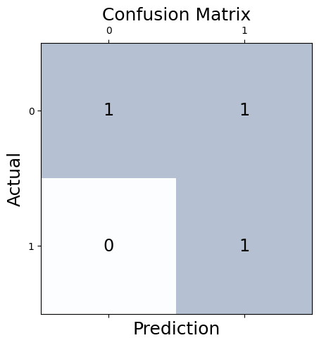
# Calculate the confusion matrix

conf_matrix = confusion_matrix(y_true=y_test, y_pred=y_pred)

# Print the confusion matrix using Matplotlib
fig, ax = plt.subplots(figsize=(5, 5))
ax.matshow(conf_matrix, cmap=plt.cm.Blues, alpha=0.3)
for i in range(conf_matrix.shape[0]):
    for j in range(conf_matrix.shape[1]):
        ax.text(x=j, y=i,s=conf_matrix[i, j], va='center', ha='center', size='xx-large')

plt.xlabel('Prediction', fontsize=18)
plt.ylabel('Actual', fontsize=18)
plt.title('Confusion Matrix', fontsize=18)
plt.show()
Output:
# Plotting the decision tree
plt.figure(figsize=(10,10))
tree.plot_tree(model,filled=True,feature_names=['feature1','feature2'], class_names=np.unique(y))
plt.show()
Output:

Explanation:
-
Accuracy: The model correctly predicted 67% of the cases.
-
Classification report: The report shows details about the performance of the model for both the classes (Cat and Dog).
-
Precision: Precision for Cat is 1, which means, out of all the cases model predicted as ‘Cat’, 100% are actually a ‘Cat’. Means, all predicted cats are actually cats.
-
Recall: Recall for Cat is 0.5, which means, out of all the actual ‘Cat’ cases, the model predicted 50% of them correctly. Means out of all cats, only 50% are detected correctly.
-
F1-score: It’s the combination of precision and recall. The F1-score for class cat is 0.5, and is useful when both the precision and recall are equally important.
-
Support: It’s the actual number of samples in the specific class.
-
-
Confusion matrix: The matrix shows the number of correctly and incorrectly classified instances for each class.
Decision tree plot: This plot shows how model made the decisions, with questions inside each node. The leaf nodes show the number of samples and the class predicted.
Post-Processing
- Feature Importance: You can check which features were most important in making decisions using model.feature_importances_\
print("\nFeature Importances:", model.feature_importances_)
- A/B Testing: Test your model with a new dataset or another model to make sure it is the best one and working correctly, before putting into production.
Hyperparameter Tuning
Fine-tune your model with hyperparameter tuning to improve its performance.
from sklearn.model_selection import GridSearchCV

# Define parameter grid
param_grid = {
    'max_depth': [2, 3, 4, 5],
    'min_samples_split': [2, 5, 10, 15],
    'min_samples_leaf': [1, 3, 5, 7]
}

# Initialize Grid Search
grid_search = GridSearchCV(DecisionTreeClassifier(random_state=42), param_grid, cv=5)

# Fit Grid Search
grid_search.fit(X_train, y_train)

# Best parameters and score
print("Best Parameters:", grid_search.best_params_)
print("Best Score:", grid_search.best_score_)

# Use the best model
best_model = grid_search.best_estimator_
y_pred = best_model.predict(X_test)

# Evaluate the model
accuracy = accuracy_score(y_test, y_pred)
print(f"Accuracy with best model: {accuracy:.2f}\n")

print("Classification Report:")
print(classification_report(y_test, y_pred))

print("\nConfusion Matrix:")
print(confusion_matrix(y_test, y_pred))


#plotting decision tree
plt.figure(figsize=(10,10))
tree.plot_tree(best_model,filled=True,feature_names=['feature1','feature2'], class_names=np.unique(y))
plt.show()
Output
UserWarning: The least populated class in y has only 2 members, which is less than n_splits=5.
  warnings.warn(


Best Parameters: {'max_depth': 2, 'min_samples_leaf': 1, 'min_samples_split': 2}
Best Score: 1.0
Accuracy with best model: 1.00

Classification Report:
              precision    recall  f1-score   support

         Cat       1.00      1.00      1.00         2
         Dog       1.00      1.00      1.00         1

    accuracy                           1.00         3
   macro avg       1.00      1.00      1.00         3
weighted avg       1.00      1.00      1.00         3


Confusion Matrix:
[[2 0]
 [0 1]]
Model Evaluation Metrics
Besides accuracy, other metrics can give you better insights:
- Accuracy: The overall percentage of correct predictions.
$$ \text{Accuracy} = \frac{\text{Number of Correct Predictions}}{\text{Total Number of Predictions}} $$
- Precision: Out of all the predicted positive cases, how many are actually positive.
$$ \text{Precision} = \frac{\text{True Positives}}{\text{True Positives + False Positives}} $$
- Recall: Of all the actual positive cases, how many were predicted correctly.
$$ \text{Recall} = \frac{\text{True Positives}}{\text{True Positives + False Negatives}} $$
- F1-Score: A balance between precision and recall.
$$ \text{F1-Score} = 2 * \frac{\text{Precision} * \text{Recall}}{\text{Precision + Recall}} $$
- Confusion Matrix: Shows a more detailed break down of right/wrong predictions for each class
- ROC Curve and AUC: (For classification) Shows the performance of the classifier at different thresholds.
Model Productionizing
Putting the model to use:
-
Save the Model: Use joblib or pickle to save your trained model.
-
Create an API: Make an API using Flask or FastAPI to use your model.
-
Cloud Deployment: Deploy it on AWS, Google Cloud, or Azure.
-
On-Premise Deployment: Deploy it on company servers if you need.
-
Testing & Monitoring: Thorough testing before going live and constant monitoring is very important.
Conclusion
Decision Trees are easy to understand and versatile. They are used in a variety of industries for various tasks. They provide a great starting point to understand machine learning, and are still being used for simpler problems where high performance is not very important. Many advanced algorithms such as Random Forest, Gradient boosting are based on the base of decision tree algorithm. Though these newer algorithms are now becoming popular, decision trees are still valuable for solving many real-world problems.
References
- Entropy in Machine Learning: https://www.geeksforgeeks.org/gini-impurity-and-entropy-in-decision-tree-ml/
- Decision tree learning: https://en.wikipedia.org/wiki/Decision_tree_learning