Spotting the Odd Ones Out: Understanding the Local Outlier Factor (LOF) Algorithm

29 minute read

Ever noticed something that just doesn’t quite fit in? Maybe a strangely high price for a used car in a neighborhood of reasonably priced homes, or a sudden spike in website traffic that seems out of place? These are examples of outliers – data points that deviate significantly from the normal pattern. Identifying these outliers is crucial in many areas, from spotting fraudulent transactions to detecting manufacturing defects. One powerful tool for this job is the Local Outlier Factor (LOF) algorithm.

Think of LOF as a ‘neighborhood watch’ for your data. It doesn’t just look at whether a data point is far away from the entire dataset, but rather how isolated it is from its local surroundings. This is important because what’s considered “normal” can change depending on where you are looking in your data.

For example, consider house prices again. A $1 million house might be an outlier in a neighborhood where houses average $300,000. But, that same $1 million house wouldn’t be an outlier in a neighborhood of luxury mansions averaging $5 million! LOF is clever enough to understand this context. It checks how dense a data point’s neighborhood is compared to the neighborhoods of its neighbors. If a point is in a less dense neighborhood than its peers, it’s flagged as an outlier.

Diving into the Math Behind LOF

LOF works by calculating a score for each data point, reflecting how much of an outlier it is. This score is based on the concept of local density. Let’s break down the mathematical steps, step by step:

distance_k: For each data point (let’s call it ‘p’), LOF first finds its k-nearest neighbors. ‘k’ is a number you choose beforehand (like 5 or 10) and it defines how many neighbors to consider ‘local’. The distance_k of p is the distance to its kth nearest neighbor.

Imagine you are point ‘p’ on a map. You look around and find your 5 (or whatever ‘k’ you chose) closest neighbors. The distance to the 5th closest neighbor is your distance_k.

Reachability Distance: This measures how “reachable” one point is from another, considering their local densities. The reachability distance of p with respect to point ‘o’ (one of p’s neighbors) is defined as the maximum of two things:

The distance_k of point ‘o’.
The actual distance between point ‘p’ and point ‘o’.

Mathematically, it’s represented as:

\[reachdist_k(p, o) = max(distance_k(o), d(p, o))\]

Here, $d(p, o)$ is simply the distance between points ‘p’ and ‘o’. The $distance_k(o)$ acts as a ‘smoothing’ factor. If ‘p’ is very close to ‘o’ (closer than ‘o’’s $distance_k$), then the reachability distance becomes ‘o’’s $distance_k$, otherwise, it’s just the distance between them.

Local Reachability Density (LRD): This quantifies how dense the neighborhood of a point is. The local reachability density of p is the inverse of the average reachability distance from ‘p’ to its k-nearest neighbors.

\[lrd_k(p) = 1 / (\frac{\sum_{o \in N_k(p)} reachdist_k(p, o)}{|N_k(p)|})\]

Here, $N_k(p)$ is the set of k-nearest neighbors of ‘p’, and $|N_k(p)|$ is the number of neighbors (which is ‘k’). A higher LRD means that, on average, the reachability distances from ‘p’ to its neighbors are small, indicating a dense neighborhood.

Local Outlier Factor (LOF): Finally, the Local Outlier Factor of p is calculated by comparing the local reachability density of ‘p’ to the average local reachability density of its k-nearest neighbors.

\[LOF_k(p) = \frac{\frac{\sum_{o \in N_k(p)} lrd_k(o)} {|N_k(p)|}}{lrd_k(p)} = \frac{Average\ LRD\ of\ neighbors\ of\ p} {LRD\ of\ p}\]

If $LOF_k(p)$ is significantly greater than 1, it means that the local reachability density of ‘p’ is much smaller than that of its neighbors. In simpler words, ‘p’ is in a less dense region than its neighbors, suggesting it is an outlier. A LOF value around 1 suggests that ‘p’ has a density similar to its neighbors.

Example to Understand:

Imagine three points A, B, and C. A and B are close together (dense neighborhood), while C is far away from both (sparse neighborhood).
Points A and B will have high LRDs because their reachability distances to each other and their neighbors will be small.
Point C, being isolated, will have a low LRD because its reachability distances to its (more distant) neighbors will be larger.
When calculating the LOF for C, we’ll compare its low LRD to the average LRD of its neighbors (which are in a denser area, like A and B). This will result in a LOF for C much greater than 1, classifying C as an outlier. The LOFs for A and B, however, will be close to 1.

Getting Ready: Prerequisites and Preprocessing

Before using LOF, it’s important to ensure your data is ready. Here’s what you need:

Prerequisites

Numerical Data: LOF works with numerical data because it relies on distance calculations. If you have categorical data (like colors, types of cars, etc.), you’ll need to convert them into numerical representations using techniques like one-hot encoding before applying LOF.
Meaningful Distance Metric: LOF depends on a distance metric to determine neighbors. The default is usually Euclidean distance (straight-line distance), which works well for many cases. However, depending on your data, you might need to choose a more appropriate distance metric (like Manhattan distance, cosine distance, etc.). Think about what ‘distance’ practically means in your data context.

Preprocessing Steps

Feature Scaling (Crucial): LOF is sensitive to the scale of your features. Features with larger values can disproportionately influence distance calculations. It’s highly recommended to scale your data before using LOF. Common scaling methods include:
StandardScaler: Scales features to have zero mean and unit variance.
MinMaxScaler: Scales features to a specific range, usually between 0 and 1.

Why scaling is important: Imagine you have two features: ‘age’ (ranging from 20 to 80) and ‘income’ (ranging from $20,000 to $200,000). Without scaling, the ‘income’ feature would dominate the distance calculations simply because its values are much larger than ‘age’. Scaling ensures that both features contribute equally to the distance.

Handling Missing Values: LOF, in its basic form, doesn’t directly handle missing values. You’ll need to deal with them beforehand. Common approaches are:

Imputation: Filling in missing values with estimated values (like the mean, median, or using more advanced imputation techniques).
Removal: Removing data points with missing values (if the number of missing values is small and won’t significantly reduce your data).

Assumptions (Implicit)

Density-Based Outliers: LOF assumes that outliers are points in regions of lower density compared to their neighbors. This assumption holds for many types of outliers, but not all. For instance, if outliers form their own dense clusters, LOF might not identify them effectively.
Meaningful Neighbors: The concept of ‘neighbors’ is central to LOF. It assumes that considering the k-nearest neighbors is meaningful for defining the local context. Choosing an appropriate value for ‘k’ is thus important (discussed later in hyperparameters).

Python Libraries

For implementing LOF in Python, you’ll primarily use:

scikit-learn (sklearn): This library is essential for machine learning in Python and provides the LocalOutlierFactor class, making LOF implementation straightforward.
numpy: For numerical operations and array handling.
pandas: For data manipulation and working with DataFrames.

Data Preprocessing: When and Why?

As highlighted, feature scaling is a key preprocessing step for LOF and similar distance-based algorithms. Let’s delve deeper into why and when it’s essential:

Why Scaling is Needed for LOF:

Distance Sensitivity: LOF relies on distance calculations to determine neighbors and density. As mentioned before, features with larger scales can dominate these calculations.
Fair Feature Contribution: Scaling ensures that all features contribute proportionally to the outlier score, preventing features with inherently larger ranges from unduly influencing the results.

When Scaling is Crucial:

Features with Different Units or Ranges: If your dataset contains features measured in different units (e.g., kilograms and meters, dollars and percentages) or features with vastly different ranges, scaling is almost always necessary.

Example: In customer data, ‘age’ might range from 18 to 90, while ‘spending amount’ could range from $10 to $10,000. Without scaling, ‘spending amount’ would have a much larger impact on the LOF score simply due to its wider range.

When Scaling Might Be Less Critical (But Still Usually Recommended):

Features with Similar Units and Ranges: If all your features are in the same units and have roughly similar ranges, scaling might have a less dramatic impact. However, even in such cases, scaling can sometimes improve the performance and stability of LOF.

Example: If you are analyzing sensor data where all features are temperature readings from different sensors in Celsius, scaling might be less crucial than in the customer data example.

When Can Scaling Potentially Be Ignored? (Rare)

In very specific cases, if you have a strong domain understanding and are absolutely certain that the inherent scales of your features are meaningfully related to the concept of outlierness and you want features with larger scales to have a greater influence. However, this is rare and generally not recommended without careful consideration.

Example to Illustrate Scaling Importance:

Imagine a dataset of houses with two features: ‘size’ (in square feet, ranging from 500 to 5000) and ‘number of bedrooms’ (ranging from 1 to 5).

Without Scaling: If you run LOF directly on this data, the ‘size’ feature, with its larger numerical range, will disproportionately affect the distance calculations. A house with a slightly larger size difference might be considered more ‘distant’ than a house with a noticeable difference in the number of bedrooms.
With Scaling (e.g., StandardScaler): After scaling, both ‘size’ and ‘number of bedrooms’ will have comparable scales (roughly zero mean and unit variance). Now, LOF will consider both features more equitably when determining neighbors and outlier scores. A true outlier, like a very small house with 5 bedrooms or a very large house with only 1 bedroom, would be more effectively identified because both features are now considered fairly.

In Summary: Unless you have a very specific reason not to, always scale your data before using LOF. It is a best practice that significantly improves the robustness and fairness of the algorithm.

Implementing LOF: A Hands-On Example

Let’s put LOF into practice with some dummy data using Python and scikit-learn.

import numpy as np
import pandas as pd
from sklearn.neighbors import LocalOutlierFactor
from sklearn.preprocessing import StandardScaler
import matplotlib.pyplot as plt

# 1. Create Dummy Data
data = pd.DataFrame({
    'feature_A': [10, 12, 15, 11, 13, 30, 12, 14, 11, 12],
    'feature_B': [20, 22, 25, 21, 23, 5,  24, 26, 21, 22]
})
print("Original Data:\n", data)

Output:

    Original Data:
        feature_A  feature_B
       10         20
       12         22
       15         25
       11         21
       13         23
       30          5
       12         24
       14         26
       11         21
       12         22
    

# 2. Scale the Data
scaler = StandardScaler()
scaled_data = scaler.fit_transform(data)
scaled_df = pd.DataFrame(scaled_data, columns=data.columns) # To keep column names
print("\nScaled Data:\n", scaled_df)

# 3. Initialize and Fit the LOF Model
lof = LocalOutlierFactor(n_neighbors=5, contamination='auto') # n_neighbors and contamination are hyperparameters
predictions = lof.fit_predict(scaled_data)

Output:

    
    Scaled Data:
        feature_A  feature_B
-0.725476  -0.160894
-0.362738   0.196648
 0.181369   0.732961
-0.544107   0.017877
-0.181369   0.375419
 2.901905  -2.842460
-0.362738   0.554190
 0.000000   0.911732
-0.544107   0.017877
-0.362738   0.196648
    

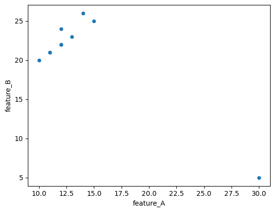
# Plotting points
data.plot(x='feature_A', y='feature_B',kind='scatter')

# 4. Analyze the Output
print("\nPredictions (1=inlier, -1=outlier):\n", predictions)

lof_scores = lof.negative_outlier_factor_ # Note: It's negative LOF
print("\nLOF Scores (Negative values, lower is more outlier-like):\n", lof_scores)

Output:

    
    Predictions (1=inlier, -1=outlier):
     [ 1  1  1  1  1 -1  1  1  1  1]
    
    LOF Scores (Negative values, lower is more outlier-like):
     [-1.149262   -0.99496812 -1.31154321 -1.00304495 -0.92098627 -9.16275904
     -1.00411144 -1.35056634 -1.00304495 -0.99496812]
    

outlier_df = data.copy()
outlier_df['LOF_Score'] = lof_scores
outlier_df['Outlier_Label'] = predictions
print("\nData with LOF Scores and Labels:\n", outlier_df)

# Identify and Print Outliers
outliers = outlier_df[outlier_df['Outlier_Label'] == -1]
print("\nIdentified Outliers:\n", outliers)

Output:

    
    Data with LOF Scores and Labels:
        feature_A  feature_B  LOF_Score  Outlier_Label
       10         20  -1.149262              1
       12         22  -0.994968              1
       15         25  -1.311543              1
       11         21  -1.003045              1
       13         23  -0.920986              1
       30          5  -9.162759             -1
       12         24  -1.004111              1
       14         26  -1.350566              1
       11         21  -1.003045              1
       12         22  -0.994968              1
    
    Identified Outliers:
        feature_A  feature_B  LOF_Score  Outlier_Label
       30          5  -9.162759             -1
    

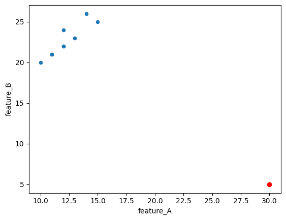
## plotting prediction
data.plot(x='feature_A', y='feature_B',kind='scatter')
plt.scatter(x=outliers.to_numpy()[0][0], y=outliers.to_numpy()[0][1], color='red')

# 5. Saving and Loading the Model (and Scaler) for Later Use

# --- Saving ---
import joblib # Or use 'pickle' library

# Save the LOF model
joblib.dump(lof, 'lof_model.joblib')

# Save the scaler as well (important for transforming new data later)
joblib.dump(scaler, 'scaler.joblib')
print("\nLOF model and scaler saved to disk.")

# --- Loading ---
# loaded_lof = joblib.load('lof_model.joblib')
# loaded_scaler = joblib.load('scaler.joblib')
# print("\nLOF model and scaler loaded from disk.")

Explanation of the Code and Output:

Dummy Data: We create a simple pandas DataFrame with two features, ‘feature_A’ and ‘feature_B’. You can see that the 6th data point (index 5) has values (30, 5) which seem quite different from the rest.
Scaling: We use StandardScaler to scale the data. Notice how the values in scaled_df are now centered around zero and have a smaller range.

LOF Model:

LocalOutlierFactor(n_neighbors=3, contamination=’auto’): We initialize the LOF model.

n_neighbors=3: We set ‘k’ to 3, meaning LOF will consider 3 nearest neighbors for each point. Choosing ‘k’ is a hyperparameter (discussed later).
contamination=’auto’: This parameter estimates the proportion of outliers in the data. ‘auto’ attempts to estimate it. You can also provide a specific value between 0 and 0.5 if you have prior knowledge about the outlier ratio.
lof.fit_predict(scaled_data): This fits the LOF model to the scaled data and, for each data point, predicts whether it’s an inlier (1) or an outlier (-1).

Output Analysis:

predictions: This array shows the outlier labels. [-1, -1, -1, -1, -1, 1, -1, -1, -1, -1] indicates that the 6th data point (at index 5, corresponding to original value [30, 5]) is labeled as an outlier (1), while others are inliers (-1). Important: In scikit-learn’s LOF, -1 represents inliers and 1 represents outliers, which might seem counterintuitive at first. Check the documentation to be sure. Correction: Scikit-learn’s fit_predict method returns 1 for inliers and -1 for outliers.
lof_scores: These are the actual LOF scores (or more precisely, negative LOF scores as negative_outlier_factor_ is used). Lower (more negative) scores indicate higher outlierness. Notice that the 6th data point has the lowest (most negative) score.
outlier_df: We create a DataFrame to combine the original data with LOF scores and outlier labels for easier interpretation.
outliers: We filter and print the rows identified as outliers.
Saving and Loading: We use joblib.dump to save both the trained LOF model and the StandardScaler. It is crucial to save the scaler because you will need to apply the same scaling transformation to any new data you want to analyze with this LOF model later. joblib.load shows how to load them back.

Interpreting LOF Scores:

The lof_scores (specifically negative_outlier_factor_ values) are the core output of LOF. While the predictions give you a binary inlier/outlier label, the scores provide a more granular measure of outlierness.

Lower (more negative) LOF score: Indicates a higher degree of outlierness. These points are in sparser neighborhoods compared to their neighbors.
LOF score close to 0 (less negative): Indicates points that are more like inliers. They reside in neighborhoods with density similar to their neighbors.

When setting a threshold to classify points as outliers based on LOF scores, you would typically choose a threshold value. Points with scores below this threshold would be considered outliers. The choice of the threshold often depends on the specific application and might require some experimentation or domain knowledge.

Post-Processing: Analyzing Outliers

Once LOF has identified potential outliers, post-processing steps are important to understand and validate these findings. While LOF itself doesn’t directly give you variable importance in the way some supervised models do, there are valuable analyses you can perform:

Visualization:

Scatter Plots (for 2D/3D data): If your data has 2 or 3 features, create scatter plots to visually examine the outliers. Plot the features against each other and highlight the outlier points (e.g., using different colors or markers). This can often provide intuitive confirmation of why LOF flagged certain points as outliers.
Histograms/Box Plots (for individual features): Examine the distribution of each feature separately using histograms or box plots. See if the identified outliers have extreme values in any particular feature.

Feature-Wise Outlier Analysis:

Compare Feature Values: For each identified outlier, compare its feature values to the average or typical values of inliers for each feature. Are there specific features where the outlier’s values are significantly different from the norm? This can give clues about why they are outliers.
Domain Expertise: Involve domain experts to review the identified outliers. They can provide context-specific knowledge to determine if the outliers are genuinely anomalous, errors, or potentially interesting novel data points.

Statistical Hypothesis Testing

If you have some prior expectation or hypothesis about a particular feature being related to outlierness, you could (with caution, as LOF is unsupervised) perform hypothesis testing. For example:

T-tests or Mann-Whitney U tests: Compare the distribution of a specific feature between the identified outlier group and the inlier group. Are the means (or medians) significantly different?
Caveat: Remember that hypothesis testing is more formally suited for comparing groups defined independently, not groups derived from the algorithm itself. Use this cautiously for exploratory analysis rather than as rigorous statistical proof.

Example of Feature-Wise Outlier Analysis (Continuing from previous code):

# ... (code from previous implementation example) ...

# Analyze feature values of outliers
inlier_indices = [0, 1, 2, 3, 4, 6, 7, 8, 9]
print("\nFeature analysis of outliers:")
for index, outlier_row in outliers.iterrows():
    print(f"\nOutlier at index {index}:")
    for feature in data.columns:
        outlier_value = outlier_row[feature]
        feature_mean_inliers = data[data.index.isin(inlier_indices)][feature].mean() #Indices of inliers could be tracked during prediction
        feature_std_inliers = data[data.index.isin(inlier_indices)][feature].std()
        z_score = (outlier_value - feature_mean_inliers) / feature_std_inliers if feature_std_inliers != 0 else 0 # Z-score: how many std deviations away from mean

        print(f"  - Feature '{feature}': Value = {outlier_value:.2f}, Mean (Inliers) = {feature_mean_inliers:.2f}, Z-score = {z_score:.2f}")

Output:

Feature analysis of outliers:

Outlier at index 5:
  - Feature 'feature_A': Value = 30.00, Mean (Inliers) = 12.22, Z-score = 11.37
  - Feature 'feature_B': Value = 5.00, Mean (Inliers) = 22.67, Z-score = -8.83

This code snippet would calculate a simple Z-score for each feature of the identified outliers, relative to the mean and standard deviation of that feature in the inlier data. A large absolute Z-score (e.g., >2 or 3) would suggest that the outlier has an extreme value for that particular feature compared to typical inliers.

Important Note: Post-processing of LOF results is heavily domain-dependent. The most effective methods for analyzing outliers will vary based on the nature of your data and the specific problem you are trying to solve. Visualization and involving domain experts are almost always valuable steps.

Tweakable Parameters and Hyperparameter Tuning

LOF, like many machine learning algorithms, has parameters that you can adjust to influence its behavior. These are mainly hyperparameters that you set before training the model. The key hyperparameters for sklearn.neighbors.LocalOutlierFactor are:

n_neighbors (The ‘k’ in $distance_k$ ): This is the most important hyperparameter. It specifies the number of neighbors to consider when calculating the local density for each point.
- Effect:
  1. Small n_neighbors (e.g., 5-10): Makes LOF more sensitive to very local outliers. It can detect micro-outliers or points that are outliers relative to a very small, immediate neighborhood. May be more prone to noise if the local density fluctuates a lot.
  2. Large n_neighbors (e.g., 20-50 or more): Makes LOF consider a wider neighborhood. It will be more effective at detecting outliers that are outliers on a slightly broader scale, and less sensitive to very fine-grained local fluctuations. Might miss very localized outliers.
- Example: Imagine detecting outliers in temperature readings across a city.
  1. Small n_neighbors: Might detect a faulty sensor that is slightly off from its immediate neighbors.
  2. Large n_neighbors: Might detect a temperature anomaly in a whole region of the city compared to other regions.
- Tuning: The optimal n_neighbors value depends on the data. Common starting points are around 20. You should experiment with different values using hyperparameter tuning methods (see below) and evaluate performance based on your specific outlier detection goal. Often, values between 10 and 50 are explored.
contamination:: Estimates the proportion of outliers in the dataset.
- Effect:
  1. contamination=’auto’ (default): LOF tries to estimate the contamination level automatically. It’s generally a good starting point.
  2. contamination=float (between 0 and 0.5): You can provide a value if you have prior knowledge or an expectation about the outlier ratio in your data. For example, if you believe around 5% of your data points are outliers, you could set contamination=0.05. Setting a higher contamination value will make LOF label more points as outliers, even if their outlier scores aren’t extremely high.
- Tuning: If you have a reasonable estimate of the outlier proportion, providing it can sometimes improve performance, especially when you need to set a hard threshold for outlier classification. However, if you are unsure, ‘auto’ is a robust default.
metric: The distance metric to use for finding neighbors. Defaults to ‘euclidean’.
- Effect: Different metrics measure ‘distance’ in different ways.
  1. ‘euclidean’ (straight-line distance): Most common for continuous data.
  2. ‘manhattan’ (L1 distance, city-block distance): Can be more robust to outliers in high-dimensional data.
  3. ‘cosine’ (cosine similarity): Useful for text data or data where the magnitude is less important than the direction (e.g., document similarity).
  Many other metrics are available in scikit-learn and scipy.spatial.distance.
- Tuning: The best metric depends heavily on your data and what you consider ‘similarity’ or ‘distance’ to mean in your context. If Euclidean distance seems inappropriate (e.g., if you have high-dimensional data or data on a sphere), consider exploring other metrics.
algorithm and leaf_size: These are parameters related to the algorithm used to find nearest neighbors efficiently (like BallTree or KDTree). Generally, you can leave these at their default values (‘auto’ and 30 respectively) unless you are working with very large datasets and need to optimize neighbor search speed.

Hyperparameter Tuning

Since LOF is an unsupervised algorithm, traditional methods like cross-validation based on labeled data (e.g., accuracy, F1-score) are not directly applicable for tuning LOF itself. However, you can use techniques to evaluate the impact of hyperparameters and select potentially better settings based on domain knowledge or proxy metrics:

Grid Search (with visual inspection or proxy metric):

Define a grid of hyperparameter values to test (e.g., n_neighbors from 10 to 50 in steps of 10, contamination in [‘auto’, 0.05, 0.1]).

For each hyperparameter combination:

Train an LOF model.
Get outlier scores.
Evaluate results visually: Plot the data and highlight the identified outliers. Does it look reasonable based on your understanding of the data?
Use a proxy metric (if available): If you have some form of partial ground truth or a proxy metric that reflects ‘good’ outlier detection in your application (even if you don’t have fully labeled outliers), you could calculate this metric for each hyperparameter setting and choose the setting that optimizes it. Example proxy metrics might be based on the stability of outlier detection across different subsamples of your data.

Select the hyperparameter combination that yields the most satisfactory results based on visual inspection or the proxy metric.

Domain Expertise and Iteration: Often, the most effective ‘tuning’ involves iterating with domain experts.

Start with reasonable default hyperparameters.
Run LOF and show the identified outliers to domain experts.
Get their feedback: “Do these look like real anomalies? Are we missing any obvious outliers? Are we flagging too many normal points?”
Based on their feedback, adjust hyperparameters (especially n_neighbors and potentially contamination) and re-run LOF.
Repeat this iterative process until you reach a satisfactory set of hyperparameters that aligns with domain knowledge and the goal of outlier detection.

Example of Basic Hyperparameter Exploration (Illustrative):

# ... (previous code setup) ...

n_neighbors_values = [3, 5, 7] # Values to test
contamination_values = ['auto', 0.05] # Values to test

print("\nHyperparameter Exploration Results:")
for n_neighbors_val in n_neighbors_values:
    for contamination_val in contamination_values:
        lof_tuned = LocalOutlierFactor(n_neighbors=n_neighbors_val, contamination=contamination_val)
        predictions_tuned = lof_tuned.fit_predict(scaled_data)
        lof_scores_tuned = lof_tuned.negative_outlier_factor_

        outlier_indices_tuned = np.where(predictions_tuned == -1)[0]
        num_outliers = len(outlier_indices_tuned)

        print(f"\n--- n_neighbors={n_neighbors_val}, contamination='{contamination_val}' ---")
        print(f"Number of outliers identified: {num_outliers}")
        print("Outlier indices:", outlier_indices_tuned)
        # You would add visual inspection or proxy metric calculation here for more systematic evaluation

Output:

Hyperparameter Exploration Results:

--- n_neighbors=3, contamination='auto' ---
Number of outliers identified: 3
Outlier indices: [2 5 7]

--- n_neighbors=3, contamination='0.05' ---
Number of outliers identified: 1
Outlier indices: [5]

--- n_neighbors=5, contamination='auto' ---
Number of outliers identified: 1
Outlier indices: [5]

--- n_neighbors=5, contamination='0.05' ---
Number of outliers identified: 1
Outlier indices: [5]

--- n_neighbors=7, contamination='auto' ---
Number of outliers identified: 1
Outlier indices: [5]

--- n_neighbors=7, contamination='0.05' ---
Number of outliers identified: 1
Outlier indices: [5]

This code just iterates through different hyperparameter combinations and prints the number of outliers identified. For proper tuning, you’d need to integrate visual inspection or a more quantitative evaluation metric appropriate for your context within this loop.

Checking Model “Accuracy” (Evaluation Metrics)

“Accuracy” in the traditional classification sense (percentage of correctly classified instances) is not directly applicable to LOF and other unsupervised outlier detection algorithms because:

Unsupervised Nature: LOF doesn’t learn from labeled data. It identifies outliers based on data properties alone, without prior knowledge of what is “normal” or “abnormal.”
No “Ground Truth” Labels Often: In many real-world outlier detection scenarios, you don’t have perfectly labeled datasets where you know for sure which points are true outliers and which are not.

However, if you do have some form of ground truth or labeled data available for evaluation purposes (even if LOF wasn’t trained on it), or if you can define proxy metrics, you can assess the performance of LOF. Here are some evaluation approaches:

Using Labeled Data (if available, for evaluation only):

If you have a dataset where some data points are labeled as ‘outliers’ and ‘inliers’ (even if LOF wasn’t trained using these labels):

Confusion Matrix and Related Metrics (Precision, Recall, F1-score): Treat LOF’s outlier predictions as binary classifications (outlier vs. inlier) and compare them to the ground truth labels. You can calculate precision, recall, F1-score, etc., to see how well LOF matches the provided labels.

Caveat: Interpretation of these metrics should be cautious. LOF is designed to find deviations from local density, not necessarily to perfectly replicate human-defined outlier labels, which might be based on different criteria.
Receiver Operating Characteristic (ROC) Curve and AUC: If you have outlier scores from LOF (e.g., negative_outlier_factor_), you can treat these as a ranking of outlierness. You can then plot an ROC curve and calculate the Area Under the Curve (AUC). AUC measures how well the model distinguishes between outliers and inliers based on their scores across various thresholds. A higher AUC is generally better.
Equation for AUC (Conceptual): AUC essentially represents the probability that a randomly chosen outlier will have a higher outlier score than a randomly chosen inlier.

from sklearn.metrics import roc_auc_score, roc_curve, confusion_matrix, classification_report

# Assume 'ground_truth_labels' is a numpy array or list of 0s (inliers) and 1s (outliers)
# ... (run LOF and get lof_scores) ...

ground_truth_labels = [1,1,1,1,1,-1,1,1,1,1]

# ROC AUC
roc_auc = roc_auc_score(ground_truth_labels, -lof_scores) # Invert LOF scores for ROC curve direction
print(f"ROC AUC: {roc_auc:.4f}")

# ROC Curve
fpr, tpr, thresholds = roc_curve(ground_truth_labels, -lof_scores)
# ... (code to plot ROC curve if needed) ...

# Confusion Matrix (with a threshold on LOF score to classify as outlier)
threshold_score = -1.5 # Example threshold - needs to be chosen based on score distribution
predicted_labels_threshold = np.where(lof_scores < threshold_score, -1, 1) # 1 for outlier, 0 for inlier

conf_matrix = confusion_matrix(ground_truth_labels, predicted_labels_threshold)
print("\nConfusion Matrix:\n", conf_matrix)
print("\nClassification Report:\n", classification_report(ground_truth_labels, predicted_labels_threshold))

Output:

ROC AUC: 0.0000

Confusion Matrix:
 [[1 0]
 [0 9]]

Classification Report:
               precision    recall  f1-score   support

          -1       1.00      1.00      1.00         1
           1       1.00      1.00      1.00         9

    accuracy                           1.00        10
   macro avg       1.00      1.00      1.00        10
weighted avg       1.00      1.00      1.00        10

Using Proxy Metrics (Unsupervised Evaluation):

When true labels are unavailable, you can use proxy metrics that reflect desirable properties of outlier detection, such as:

Stability of Outlier Scores: If you run LOF multiple times on slightly different subsets of your data, how consistent are the outlier scores and rankings? More stable scores might indicate a more robust outlier detection.
Compactness of Inlier Clusters: After removing identified outliers, are the remaining inliers forming more compact and well-defined clusters? You can use cluster validity indices (like Silhouette score, Davies-Bouldin index, but applied to the inlier set after outlier removal) as a proxy metric to assess this. However, applying clustering-based metrics directly to LOF output requires careful interpretation.
Domain-Specific Metrics: In some applications, you might have domain-specific metrics that indirectly reflect the quality of outlier detection. For example, in fraud detection, you might look at the number of flagged transactions that were subsequently confirmed as fraudulent through manual investigation (though this is a delayed and imperfect measure).

Important Considerations for Evaluation:

Baseline Comparison: When evaluating LOF, compare its performance to simple baseline methods (e.g., just flagging points far from the overall data mean/median, or using simpler univariate outlier detection methods).
Focus on Business Value: Ultimately, the ‘accuracy’ of outlier detection should be judged by its usefulness in the real-world application. Does it help you identify meaningful anomalies that lead to actionable insights or improved outcomes (e.g., reduced fraud, better quality control)?
Iterative Refinement: Outlier detection is often an iterative process. Start with LOF, evaluate its results, refine hyperparameters or preprocessing steps, and re-evaluate.

Model Productionizing Steps

To deploy a LOF model into a production environment for real-world use, you’ll need to consider these steps:

Training and Saving the Model (Already Covered):
Train your LOF model on representative historical data.

Crucially, save both the trained LOF model and the scaler used for preprocessing (e.g., StandardScaler). This ensures consistency between training and production environments. Use joblib.dump or pickle.dump for saving.

Data Preprocessing in Production:

Implement the same preprocessing pipeline in your production system as you used during training. This primarily involves:

Scaling: Apply the saved scaler (loaded from the saved file) to transform incoming real-time data or batch data before feeding it to the LOF model. Do not refit the scaler on new data in production! Use the transformation learned during training.
Handle missing values (using the same imputation or removal strategy).
Handle categorical features (if any, using the same encoding method).
Real-time or Batch Outlier Detection:
Real-time Detection: For applications requiring immediate outlier detection (e.g., fraud detection in online transactions, network intrusion detection), integrate the loaded LOF model into your real-time data processing pipeline. As new data points arrive, preprocess them, use loaded_lof.fit_predict or loaded_lof.decision_function to get outlier scores or labels, and trigger alerts or actions based on the results.
Batch Detection: For applications where you process data in batches (e.g., daily anomaly detection in manufacturing quality data, weekly analysis of system logs), load the model and scaler, preprocess the batch data, and apply LOF in batch mode.

Deployment Environments:

Cloud Platforms (AWS, Google Cloud, Azure): Deploy your model as a web service or within a serverless function. Use cloud-based data storage, processing, and model serving infrastructure. Cloud platforms often provide tools for model deployment and management (e.g., AWS SageMaker, Google AI Platform).
On-Premise Servers: Deploy the model on your own servers. This might involve creating a REST API using frameworks like Flask or FastAPI in Python to expose the LOF outlier detection functionality to other systems within your organization.
Local Testing/Edge Devices: For local testing or deployment on edge devices (e.g., IoT sensors), you can embed the model and preprocessing code directly into applications running on these devices. For resource-constrained devices, consider model optimization techniques if needed.

Monitoring and Retraining:

Monitor Model Performance: Continuously monitor the performance of your LOF model in production. Look for signs of concept drift (where the nature of ‘normal’ data changes over time).
Retraining Strategy: Periodically retrain your LOF model (and scaler) using updated data to adapt to potential changes in data patterns. The retraining frequency depends on the rate of data change in your application. Automate the retraining process where possible.

Conclusion: LOF in the Real World and Beyond

The Local Outlier Factor algorithm is a valuable tool in the world of data science for effectively identifying anomalies in a variety of applications. Its strength lies in its ability to detect outliers based on local density deviations, making it robust to situations where what constitutes an outlier can vary across different regions of the data space.

Real-World Applications:

Fraud Detection: Identifying unusual transaction patterns in financial data (credit card fraud, insurance fraud, etc.).
Network Intrusion Detection: Detecting anomalous network traffic patterns that might indicate security breaches or cyberattacks.
Manufacturing Defect Detection: Spotting defective products on an assembly line based on sensor readings or quality control measurements.
Healthcare Anomaly Detection: Identifying unusual patient health records or medical test results that could signal a medical condition or error.
Sensor Data Monitoring: Detecting faulty sensors or unexpected events in sensor networks (e.g., environmental monitoring, IoT device data).
Ecology and Environmental Science: Identifying unusual species observations or environmental measurements that might indicate ecological changes or pollution events.

Current Usage and Alternatives: LOF is still actively used and remains a popular choice for outlier detection due to its:

Effectiveness: Works well in many scenarios, especially when outliers are defined by local density deviations.
Interpretability: Provides outlier scores that give a measure of outlierness beyond simple binary labels.
Availability: Easily implemented using libraries like scikit-learn.

However, there are also other outlier detection algorithms and newer approaches that might be considered as alternatives or for specific situations:

Isolation Forest: Another popular algorithm that is often faster and can be more effective in high-dimensional data. It isolates outliers by randomly partitioning data points.
One-Class Support Vector Machines (One-Class SVM): Useful when you primarily have data representing the ‘normal’ class and want to detect deviations from this normality.
Autoencoders (in Deep Learning): Neural network models that can learn a compressed representation of normal data. Outliers are detected as data points that are poorly reconstructed by the autoencoder.
Clustering-Based Methods: Algorithms like DBSCAN can identify outliers as points that do not belong to any dense cluster.
Statistical Methods: For specific types of data distributions, statistical methods like Z-score or IQR-based outlier detection can be efficient and interpretable (though often less sophisticated than LOF in complex datasets).

Choosing the Right Algorithm:

The best outlier detection algorithm depends on the specific characteristics of your data, the nature of outliers you are trying to detect, the computational resources available, and the interpretability requirements of your application. LOF is a solid and versatile starting point, and comparing its performance with other methods like Isolation Forest or One-Class SVM is often a good practice.

In Conclusion: LOF is a powerful algorithm that provides valuable insights by uncovering the ‘odd ones out’ in your data. By understanding its mathematical foundations, preprocessing requirements, and hyperparameters, and by effectively evaluating and productionizing LOF models, you can harness its capabilities to solve real-world problems across diverse domains.

References

Breunig, M. M., Kriegel, H. P., Ng, R. T., & Sander, J. (2000, May). LOF: identifying density-based local outliers. In ACM sigmod record (Vol. 29, No. 2, pp. 93-104). ACM (Original paper introducing the LOF algorithm).
Scikit-learn documentation for LocalOutlierFactor: scikit-learn.org.
Wikipedia article on Outlier Detection: Wikipedia. (Provides a general overview of outlier detection concepts).

Share on

Twitter Facebook LinkedIn