Isolation Forest: Finding Needles in a Haystack
Have you ever wondered how banks detect fraudulent transactions, or how manufacturers identify faulty products on an assembly line? These are real-world problems where we need to find the “odd ones out” – the anomalies. One powerful tool for this is the Isolation Forest algorithm. Let’s dive in and see what it’s all about!
What is Anomaly Detection?
Imagine you’re looking at a field of green grass. Suddenly, you spot a bright red flower. That red flower stands out because it’s different from the rest. In data science, “anomalies” or “outliers” are data points that are different from the majority of your data.
Real-World Examples:
- Credit Card Fraud: When someone uses your credit card in a location you’ve never been to, it’s flagged as an anomaly.
- Manufacturing Defects: A product that doesn’t meet quality standards during manufacturing is an anomaly.
- Network Security: A sudden surge in network traffic that is unusual is an anomaly that may indicate a cyberattack.
- Medical Diagnosis: An unusual measurement in a patient’s blood test could indicate an illness.
How Does Isolation Forest Work?
The Isolation Forest algorithm takes a very unique approach to finding these oddities. Instead of trying to profile ‘normal’ data, it focuses on directly isolating ‘anomalous’ data points. Here’s the basic idea:
- Random Partitioning: The algorithm randomly selects a feature (a column in your data) and then randomly picks a split value within the range of that feature. Think of it like cutting a cake into slices using random cuts.
- Isolation: This process is repeated to ‘separate’ or ‘isolate’ data points.
- Anomalies are Easier to Isolate: Data points that are anomalous will generally get isolated much faster – they are like small, easy-to-pick-out pieces of cake compared to larger, more complex chunks. Normal data points require more splits to be isolated.
- Path Length: The algorithm measures the number of splits it took to isolate a point. This is called the “path length”. Shorter paths indicate anomalies.
The Mathematics Behind It (Simplified)
Let’s simplify the math without getting lost in complicated equations. The main concept involves calculating the average path length and the anomaly score.
-
Path Length (h(x)): Imagine each data point as a point in a data space (think of a dot in a room). The number of splits required to isolate the point (or put a box around the point) is its path length. Anomalies will have shorter path lengths.
-
Average Path Length (c(n)): If we had to isolate n points, this is average path length. We don’t need to worry about the exact value but you can see it as the average path length required to isolate points.
-
Anomaly Score (s(x, n)): This score is calculated from the path length. Think of it as a score for how abnormal the point is.
The anomaly score is given by the formula:
\[s(x, n) = 2^{-\frac{E(h(x))}{c(n)}}\]Where:
-
s(x,n) is the anomaly score of data point x in a dataset of size n.
-
E(h(x)) is the average path length for data point x.
-
c(n) is the average path length needed to isolate a data point in a dataset of size n
Let’s break this down:
-
2 raised to something: Imagine you are playing a game where you get 2 points for each level up. So if you go up 2 levels you have 2*2 = 4 points or 2 raised to power of 2.
-
Negative Power: If we get 2 points for going up, we can say we go down by dividing the points. In this case it is just dividing by 2. So -1 means we divide by 2. -2 means we divide by 2, and again by 2, or 4.
-
E(h(x))/c(n): We already know what E(h(x)) and c(n) is. We can consider it as some number divided by other number.
-
Putting it Together: If the path length E(h(x)) is very small, then the whole fraction is small. If we have a negative of that number then the number increases, so the value \(2^{-\\frac{E(h(x))}{c(n)}} \) increase to close to 1. Which means, it is highly likely an anomaly.
In simple terms: The formula calculates a score between 0 and 1. If the score is closer to 1, the data point is likely an anomaly. If it’s close to 0, the data point is considered normal.
Prerequisites for Using Isolation Forest
Before implementing the algorithm, here are a few things to consider:
-
No Strong Assumptions: Isolation Forest makes fewer assumptions about the data distribution than many other anomaly detection methods. You don’t need to assume your data is normally distributed.
-
Numerical Data: The algorithm works best with numerical data. If you have categorical data, you’ll need to encode it into numerical form.
-
No Prior Labeling: Isolation Forest is an unsupervised learning algorithm. This means you don’t need to have labeled “normal” and “anomaly” data to train your model.
-
You can install these with pip using:
-
scikit-learn for the Isolation Forest implementation.
-
numpy for numerical operations.
-
pandas for data manipulation.
-
matplotlib and seaborn for visualization.
pip install scikit-learn numpy pandas matplotlib seaborn -
Tweakable Parameters and Hyperparameters
Here are some important parameters you can adjust in your Isolation Forest model:
-
n_estimators: The number of isolation trees to build.
-
Effect: More trees can lead to more robust results, but may also increase computational time.
-
Example: If you have very complex data with lots of outliers, increase n_estimators.
-
-
max_samples: The number of data points to use to build each tree.
-
Effect: Increasing this value can make the model better at detecting more global outliers, but less sensitive to local outliers.
-
Example: For a dataset with many global and fewer local outliers, try setting max_samples close to the size of the dataset.
-
-
contamination: The proportion of outliers you expect in your data.
-
Effect: Affects the threshold for deciding whether a point is an anomaly or not.
-
Example: If you know your data has about 5% outliers, set contamination=0.05.
-
-
max_features: The maximum number of features to consider when making a split in each tree.
-
Effect: If your dataset has too many features, then you can limit the features. If set to 1, then the tree will only use single feature.
-
Example: If you want the algorithm to use some of the features but not all of them you can limit it.
-
-
random_state: For reproducible results.
-
Effect: Setting a random state ensures that your results are consistent every time you run your code.
-
Example: Set random_state=42 for consistent results.
-
Data Preprocessing
Isolation Forest generally does not require extensive data preprocessing like data normalization, but here are some things to consider:
-
Feature Scaling: Feature scaling (like normalization or standardization) is usually not necessary because Isolation Forest uses random splits. However, if different features have very different scales, consider scaling if it increases the model performance.
-
Categorical Data Encoding: As mentioned before, you need to convert categorical features into numerical values using techniques like One-Hot Encoding or Label Encoding.
-
Handling Missing Values: Missing values can disrupt the algorithm. You might need to impute missing values using techniques like mean imputation or median imputation.
-
Feature Selection: Selecting relevant features can improve the model and reduce training time.
Example of Preprocessing: Suppose you have a dataset with student data, including age and grade_level. Age is a numeric feature that may vary from 5 to 25. Grade_level may have the value K, 1, 2, 3, 4, 5, 6, 7, 8, 9, 10, 11, 12.
In this case you can one hot encode the Grade_level feature into 13 individual features, for the values K, 1, 2, …, 12. You can ignore scaling for age column. But it is not required.
Implementation Example
Let’s implement Isolation Forest using some dummy data.
import numpy as np
import pandas as pd
from sklearn.ensemble import IsolationForest
import matplotlib.pyplot as plt
import seaborn as sns
# Generate some dummy data with anomalies
rng = np.random.RandomState(42)
X = 0.3 * rng.randn(100, 2)
X_outliers = rng.uniform(low=-4, high=4, size=(20, 2))
X = np.concatenate([X, X_outliers], axis=0)
# Create a dataframe
df = pd.DataFrame(X, columns=['feature_1', 'feature_2'])
df.head()
output
| feature_1 | feature_2 | |
|---|---|---|
| 0 | 0.149014 | -0.041479 |
| 1 | 0.194307 | 0.456909 |
| 2 | -0.070246 | -0.070241 |
| 3 | 0.473764 | 0.230230 |
| 4 | -0.140842 | 0.162768 |
# Fit Isolation Forest model
model = IsolationForest(n_estimators=100, random_state=42, contamination=0.17)
model.fit(df)
IsolationForest(contamination=0.17, random_state=42)In a Jupyter environment, please rerun this cell to show the HTML representation or trust the notebook.
On GitHub, the HTML representation is unable to render, please try loading this page with nbviewer.org.
IsolationForest(contamination=0.17, random_state=42)
# Get the anomaly scores
scores = model.decision_function(df)
# Get the anomaly prediction (1 for normal, -1 for anomaly)
predictions = model.predict(df)
# Add predictions to the DataFrame
df['anomaly_score'] = scores
df['is_anomaly'] = predictions
# Visualize results
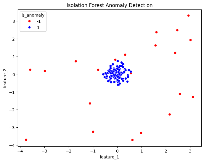
plt.figure(figsize=(8, 6))
sns.scatterplot(x='feature_1', y='feature_2', hue='is_anomaly', data=df, palette={1:'blue', -1:'red'})
plt.title('Isolation Forest Anomaly Detection')
plt.show()
# Print anomaly counts
print(df.is_anomaly.value_counts())
output
    is_anomaly
     1    99
    -1    21
    Name: count, dtype: int64
Output and Explanation:
-
Dummy data creation: We created a dummy dataset using np.random.RandomState(42) which will generate random numbers always the same if initialized with same random state. This allows for reproducibility. We generated 100 data points that are normal and 20 outliers.
-
Model Fitting: We create a IsolationForest model and fit the model using the dummy data. We used n_estimators=100 and contamination = 0.17. This is because we know that there are about 20/120=0.17 outliers.
-
Anomaly Scores: The decision_function returns the anomaly scores. The output will be between 0 to 1, and lower scores indicate anomalies.
-
Anomaly Predictions: The predict function outputs 1 for normal and -1 for anomaly.
-
Visualization: The scatter plot shows that the outliers (red) are separated from the normal data points (blue).
-
Print Anomaly Counts: The output will print how many anomalies (-1) and normal data points (1) are detected. For example:
Post-Processing and Model Evaluation
After training your model, it’s helpful to analyze results:
-
Feature Importance: Isolation Forest doesn’t directly give feature importance, but you can analyze which features are frequently used in the splits and potentially affect outlier scores. For example, if the same feature is frequently used then that feature is a good predictor.
-
Anomaly Threshold: The decision boundary is automatically set by contamination. You might want to experiment with different contamination settings.
-
A/B Testing: If your system has an intervention, you can compare its effectiveness on populations with detected anomalies versus populations without detected anomalies.
-
Since Isolation Forest is unsupervised, traditional metrics like accuracy may not be appropriate. Here are some alternative metrics:
-
Precision, Recall, F1-Score (with ground truth): If you have some known anomalies, you can calculate these scores by treating the problem as a binary classification problem. If you do not have ground truth, you can ignore it.
-
Precision = TP/(TP+FP). (True positive / true positive + false positive). Out of all the points you marked as anomaly, how many are actually an anomaly.
-
Recall = TP/(TP+FN). (True positive/ true positive + false negative). Out of all the actual anomalies, how many you identified.
-
F1-Score = 2*(Precision*Recall)/(Precision+Recall). F1 score is the harmonic mean of precision and recall.
-
Area Under the ROC Curve (AUC-ROC): If you have some known anomalies, you can plot ROC curve and calculate the AUC.
-
Qualitative Assessment: Examine the specific instances that the algorithm flags as anomalies, this can be useful in determining if the model is performing well in specific scenario.
-
Hyperparameter Tuning
Hyperparameter tuning involves systematically finding the best parameters. Here’s how to do it using GridSearchCV from scikit-learn:
from sklearn.model_selection import GridSearchCV
from sklearn.ensemble import IsolationForest

# Define the parameter grid
param_grid = {
    'n_estimators': [50, 100, 150],
    'max_samples': ['auto', 0.5, 0.8],
    'contamination': [0.10, 0.15, 0.20]
}

# Create Isolation Forest model
iso_forest = IsolationForest(random_state=42)

# Set up grid search
grid_search = GridSearchCV(estimator=iso_forest, param_grid=param_grid, cv=3, scoring='neg_mean_absolute_error')

# Fit the grid search
grid_search.fit(df[['feature_1', 'feature_2']])

# Print the best parameters
print("Best parameters found: ", grid_search.best_params_)
Output
Best parameters found: {'contamination': 0.1, 'max_samples': 'auto', 'n_estimators': 50}
grid_search.predict(df)
Output
    array([ 1,  1,  1,  1,  1,  1,  1,  1,  1,  1,  1,  1,  1,  1,  1,  1,  1,
            1,  1,  1,  1,  1,  1,  1,  1,  1,  1,  1,  1,  1,  1,  1,  1,  1,
            1,  1,  1,  1,  1,  1,  1,  1,  1,  1,  1,  1,  1,  1,  1,  1,  1,
            1,  1,  1,  1,  1,  1,  1,  1,  1,  1,  1,  1,  1,  1,  1,  1,  1,
            1,  1,  1,  1,  1,  1,  1,  1,  1,  1,  1,  1,  1,  1,  1,  1,  1,
            1,  1,  1,  1,  1,  1,  1,  1,  1,  1,  1,  1,  1,  1,  1, -1,  1,
           -1, -1, -1,  1,  1,  1, -1, -1, -1,  1,  1, -1, -1,  1, -1, -1, -1,
            1])
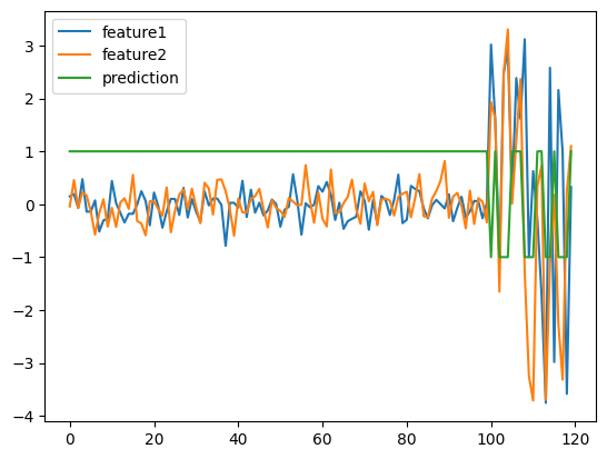
plt.plot(df)
plt.plot(grid_search.predict(df))
plt.legend(['feature1','feature2','prediction'])
Model Productionizing
Here are the steps to deploy the trained Isolation Forest model:
-
Local Testing: You can use the model on your local machine using python.
-
Cloud Deployment:
-
AWS, GCP, Azure: You can deploy the model as an API endpoint using a cloud platform’s machine learning services.
-
Docker: Containerize the model for easier deployment.
-
-
On-Premise:
- Dedicated Server: Deploy the model on a dedicated server, with an API or scheduler.
Conclusion
Isolation Forest is a powerful, versatile, and efficient algorithm for anomaly detection. Its ability to isolate anomalies directly makes it a good choice, and is being used in various industries like fraud detection, network security, and manufacturing.
While Isolation Forest has limitations, its ease of use, performance, and interpretability have cemented its place as a valuable tool. There are newer anomaly detection algorithms such as Autoencoders, and GAN-based anomaly detection, that provide better performance, depending on the use case.
Hopefully, this guide has demystified Isolation Forest and shown you how useful it can be in your projects.