Fast MCD Algorithm: A Robust Approach to Outlier Detection

Introduction to Fast MCD: Finding Needles in a Haystack, Robustly!

Imagine you are analyzing data - maybe it’s financial transactions to detect fraud, sensor readings from a machine to predict failures, or even patient data to identify unusual health patterns. In many real-world datasets, you’ll encounter outliers – data points that are significantly different from the rest. These outliers can be due to errors, anomalies, or genuinely unusual events.

Think about it like this:

• Fraud Detection in Banking: Most bank transactions are normal. But a few might be fraudulent – unusually large amounts, transactions from strange locations, etc. These fraudulent transactions are outliers.
• Manufacturing Quality Control: Most products coming off a production line are within specifications. But some might be defective – too heavy, too large, etc. These defective products represent outliers in the measurements.
• Network Security: Internet traffic is generally predictable. But hacking attempts or network failures can cause unusual patterns in traffic data – sudden spikes in activity, connections to unusual servers. These unusual patterns are outliers.

Why is finding outliers important?

• Improved Accuracy: Outliers can skew statistical analyses and machine learning models. Removing or mitigating their influence often leads to more accurate results.
• Anomaly Detection: In many cases, the outliers are the interesting points. Fraud, defects, and security breaches are all outliers we want to detect!
• Data Cleaning: Outliers can indicate data errors that need to be corrected or investigated.

Enter the Fast MCD Algorithm!

Fast Minimum Covariance Determinant (Fast MCD) is a powerful statistical technique used to identify outliers in datasets, especially when the data has multiple dimensions (many columns or features). It’s particularly useful because it’s robust. “Robust” in statistics means that the algorithm isn’t easily thrown off by the outliers it’s trying to detect. Many standard methods for finding averages and spreads in data are heavily influenced by outliers. Fast MCD is designed to be less sensitive to these extreme values.

In simple terms, Fast MCD tries to find a ‘core’ group of data points that are most similar to each other and then flags data points that are far away from this core as outliers. It does this in a clever way that’s computationally efficient, hence the “Fast” part.

The Mathematics Behind Fast MCD: Finding the Robust Center and Shape

To understand how Fast MCD works, we need to touch upon a few mathematical concepts. Don’t worry, we’ll keep it as simple as possible!

At its heart, Fast MCD is about finding a robust estimate of the covariance of your data. Let’s break this down:

• Covariance: Covariance measures how variables in your dataset change together. For example, in house prices, the size of the house and the price are likely to have a positive covariance – as size increases, price tends to increase too. The covariance matrix is a table that shows the covariance between all pairs of variables in your dataset.

  Mathematically, the covariance between two variables \(X\) and \(Y\) is often denoted as \(Cov(X, Y)\) and calculated (for a sample) as:

  \[Cov(X, Y) = \frac{\sum_{i=1}^{n} (x_i - \bar{x})(y_i - \bar{y})}{n-1}\]

  Where:

  • \(x_i\) and \(y_i\) are the individual data points for variables X and Y.
  • \(\bar{x}\) and \(\bar{y}\) are the means (averages) of variables X and Y.
  • \(n\) is the number of data points.

  For a dataset with multiple variables, we calculate the covariance between each pair of variables and arrange them in a matrix, called the covariance matrix.

• Determinant: The determinant is a value that can be calculated from a square matrix (like a covariance matrix). It provides information about the ‘volume’ spanned by the data in the space defined by your variables. In simpler terms, for a 2x2 covariance matrix, the determinant is related to the area of the ellipse that would enclose the ‘typical’ data points. A smaller determinant generally indicates a more tightly clustered dataset.

  For a 2x2 matrix \(A = \begin{pmatrix} a & b \\ c & d \end{pmatrix}\), the determinant is:

  \[det(A) = ad - bc\]

• Minimum Covariance Determinant (MCD): The MCD method tries to find a subset of your data (say, half of it or some fraction) such that if you calculate the covariance matrix just from this subset, the determinant of this covariance matrix is minimized.

  Why minimize the determinant? A smaller determinant implies that the selected subset of data is more tightly clustered and has less ‘spread’. The idea is that this tightly clustered subset represents the ‘good’ data, free from outliers. The data points not in this subset are then flagged as potential outliers.

• Fast MCD Algorithm: Calculating the MCD exactly can be computationally expensive, especially for large datasets. The “Fast MCD” algorithm is an approximation that is much quicker. It uses an iterative approach. It starts with a random subset of data, calculates its covariance and determinant, and then iteratively refines the subset to further minimize the determinant. This is done using a process called C-steps (Concentration steps). Essentially, it keeps swapping data points in and out of the subset to find a subset that gives a smaller and smaller covariance determinant.

Example to Visualize:

Imagine you have data points scattered on a 2D graph. Most points form a nice ellipse shape, but a few are scattered far away.

1. Standard Covariance: If you calculate the covariance of all points, the outliers will pull the ‘ellipse’ of covariance outwards, making it larger and more spread out.
2. MCD Covariance: MCD will try to find an ellipse that fits the main cluster of points, ignoring the outliers. The determinant of the covariance matrix for this MCD ellipse will be smaller than the determinant of the covariance matrix calculated from all data points.

Fast MCD helps us to robustly estimate the center (mean) and shape (covariance) of the ‘good’ data, effectively ignoring the influence of outliers during this estimation process.

Prerequisites and Setup for Fast MCD

Before using Fast MCD, let’s consider a few things:

Assumptions:

• Numerical Data: Fast MCD works with numerical data. If you have categorical features, you’ll need to convert them into numerical representations (e.g., using one-hot encoding) or use other outlier detection methods that are suitable for categorical data.
• Multivariate Data: While you can technically use it on one-dimensional data, MCD is most useful when you have data with multiple features or dimensions. It leverages the relationships between features to identify outliers.
• Outliers Exist (Potentially): The algorithm is designed to be effective in the presence of outliers. If you’re certain your data is perfectly clean and outlier-free, MCD might still work but might be overkill.
• No Strict Distribution Assumption: While traditional MCD methods sometimes assume data is roughly multivariate Gaussian (normally distributed in multiple dimensions), Fast MCD is reasonably robust to deviations from perfect normality. It’s more about finding a ‘core’ of consistent data than strictly fitting a Gaussian.

Testing Assumptions (Informally):

• Visual Inspection:
  • Histograms and Boxplots (for each feature): Look for long tails or extreme values in histograms and points far outside the whiskers in boxplots. These can indicate potential outliers in individual features.
  • Scatter Plots (for pairs of features): If you have 2 or 3 features, scatter plots can help you visually identify points that are far away from the main clusters.
• No Formal Pre-tests Needed: For Fast MCD, you don’t usually need to perform formal statistical tests to ‘check’ assumptions before applying it. The algorithm is designed to be robust even if the assumptions are not perfectly met. The visual checks are more for understanding your data and anticipating potential issues.

Python Libraries:

For implementing Fast MCD in Python, the primary library you’ll use is scikit-learn (sklearn). It provides an efficient implementation:

from sklearn.covariance import fast_mcd

Make sure you have scikit-learn installed. If not, you can install it using pip:

pip install scikit-learn

Data Preprocessing for Fast MCD: To Normalize or Not to Normalize?

Data preprocessing is an important step in many machine learning tasks. For Fast MCD, the need for preprocessing is less critical compared to some other algorithms, but it’s still worth considering.

Normalization/Scaling:

• Generally Not Essential: Fast MCD is based on covariance, which is somewhat scale-invariant. This means that if you multiply all values in a feature by a constant factor, the shape of the covariance structure doesn’t fundamentally change, although the magnitude of covariance values will change. Therefore, data normalization (like standardization or min-max scaling) is usually not strictly required for Fast MCD to work.

• Why it Might Help (Sometimes):
  • Features with Vastly Different Scales: If you have features with extremely different scales (e.g., one feature ranges from 0 to 1, and another ranges from 0 to 1,000,000), it could potentially influence the algorithm’s convergence or numerical stability in some cases. Scaling features to a similar range might help in such situations, although it’s not guaranteed.
  • Interpretation: If you plan to compare the “importance” or contribution of different features after outlier detection (though this isn’t the primary goal of MCD), scaling can make features more directly comparable.
• Why it Can Often Be Ignored:
  • Robustness to Scale: MCD’s robustness property extends to being less sensitive to the scale of features compared to distance-based methods like k-means clustering or k-nearest neighbors, where feature scaling is often crucial.
  • Focus on Shape, Not Magnitude: MCD primarily focuses on the shape of the data cloud (captured by the covariance matrix) and finding a robust estimate of this shape, which is less directly affected by feature scaling than measures based on distances or magnitudes.

Examples where Scaling Might Be Considered:

• Genomics Data: Gene expression data can sometimes have features (genes) with very different ranges of expression levels. In such cases, scaling might be considered as a precautionary step.
• Sensor Data with Mixed Units: If you combine sensor readings with different physical units (e.g., temperature in Celsius, pressure in Pascals, flow rate in liters per minute), and the numerical ranges are vastly different, scaling could be beneficial.

Examples where Scaling Can Usually Be Ignored:

• Financial Data (e.g., stock prices, trading volumes): While feature ranges might vary, scaling is often not a mandatory step for MCD in this domain.
• Basic Machine Learning Datasets: For many standard datasets used in machine learning examples, scaling before applying Fast MCD is often not necessary and may not significantly change the results.

In practice: Start by trying Fast MCD without scaling your data. If you encounter issues or have features with extremely disparate scales, you can then experiment with scaling (e.g., StandardScaler from scikit-learn) and see if it improves the outlier detection results or algorithm performance in your specific case. But for many scenarios, especially when using Fast MCD for initial outlier detection, scaling is not a critical preprocessing step.

Implementation Example: Outlier Detection with Fast MCD

Let’s see Fast MCD in action with a simple Python example using dummy data.

import numpy as np
from sklearn.covariance import fast_mcd
import matplotlib.pyplot as plt

# 1. Generate Dummy Data with Outliers
rng = np.random.RandomState(42) # for reproducibility
n_samples = 200
n_outliers = 25
n_features = 2

# Generate inlier data (majority of data)
data = rng.randn(n_samples, n_features)
inlier_covariance = np.eye(n_features) * 2  # Identity matrix scaled
inlier_mean = np.zeros(n_features)
inliers = np.dot(rng.randn(n_samples, n_features), inlier_covariance) + inlier_mean
data[:n_samples] = inliers

# Add outliers (making them distinct in feature space)
outlier_covariance = np.diag([5, 0.1]) # Elongated ellipse
outlier_mean = [5, 5]
outliers = np.dot(rng.randn(n_outliers, n_features), outlier_covariance) + outlier_mean
data = np.concatenate([data,outliers])

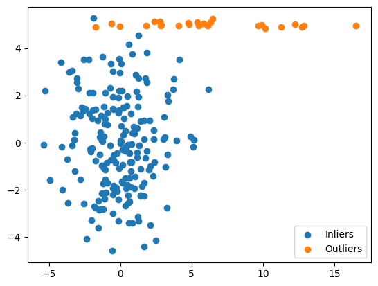
## Plotting the points
plt.scatter(*zip(*inliers))
plt.scatter(*zip(*outliers))
plt.legend(['Inliers','Outliers'])

Output:

# 2. Apply FastMCD
 # support_fraction: roughly expect 10% outliers
fast_mcd_model = fast_mcd(data, random_state=rng, support_fraction=0.9)
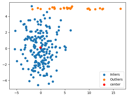
## plotting the center of fast mcd
plt.scatter(*zip(*inliers))
plt.scatter(*zip(*outliers))
plt.scatter(*zip(fast_mcd_model[0]), color='red')
plt.legend(['Inliers','Outliers','center'])

Outout:

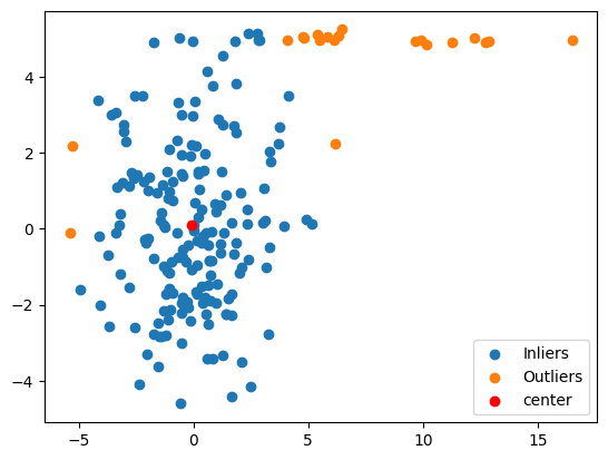
## Filtering points 
good = [v for b, v in zip(fast_mcd_model[2], data) if b]
bad = [v for b, v in zip(fast_mcd_model[2], data) if not b]

## plotting the good and bad/outliers
plt.scatter(*zip(*good))
plt.scatter(*zip(*bad))
plt.scatter(*zip(fast_mcd_model[0]), color='red')
plt.legend(['Inliers','Outliers','center'])

Output:

Explanation of the Code and Output:

1. Data Generation: We create dummy 2D data. Most of it is generated from a normal distribution (inliers), and we add a smaller number of points (outliers) that are generated to be significantly different in terms of their distribution (different mean and covariance structure).

2. FastMCD Initialization and Fitting:
   • fast_mcd(data, random_state=rng, support_fraction=0.7): We create a fast_mcd object. Add the data. random_state ensures consistent results if you re-run the code. support_fraction=0.9 is a key parameter. It tells Fast MCD to try to find a ‘core’ subset of roughly 90% of the data and consider the rest as potential outliers. Choosing support_fraction depends on your expectation of the percentage of outliers in your data. If you expect more outliers, use a lower support_fraction.
3. Getting Results:
   • robust_covariance = fast_mcd_model[1]: This gives you the robustly estimated covariance matrix calculated from the ‘inlier’ subset found by Fast MCD.
   • robust_location = fast_mcd_model[0]: This is the robust estimate of the mean (center) of the inlier data.
   • support_mask = fast_mcd_model[2]: This is a boolean array. It has True for data points that Fast MCD considers to be inliers (part of the ‘support set’) and False for outliers.

4. Separating Data: We use the support_mask to separate our original data into inlier_data and outlier_data.

5. Visualization (Optional): If you have matplotlib installed, the code will create a scatter plot showing the inliers in blue and outliers in red. This is a helpful way to visually verify if Fast MCD has identified outliers as you expected.

Output Interpretation:

When you run the code, you’ll see output similar to this (the exact numbers might vary slightly due to randomness, but the overall pattern will be the same):

Robust Covariance Matrix:
[[3.83506641, 0.31904764],
[0.31904764, 4.82047283]]

Robust Location (Mean):
 [-0.07342507,  0.10545782]

Number of Inliers Detected: 175
Number of Outliers Detected: 25

• Robust Covariance Matrix: This is the estimated covariance matrix based on the inlier data. Notice that it’s close to the inlier_covariance we used to generate the inliers ( [[2, 0], [0, 2]] in our example). This shows Fast MCD effectively estimates the covariance structure of the ‘good’ data while being less influenced by outliers.

• Robust Location (Mean): This is the estimated mean (center) of the inlier data. It’s close to inlier_mean ([0, 0]) we used for inliers.

• Number of Inliers/Outliers Detected: This tells you how many data points were classified as inliers and outliers. In our example, it correctly identifies close to 175 inliers and 25 outliers, matching our data generation process.

‘Robustness in Output:

In Fast MCD:

• Robustness is reflected in the covariance_, location_, and support_mask_ outputs themselves. These estimates are robust because they are calculated in a way that minimizes the influence of outliers.
• The support_fraction parameter indirectly controls the robustness. A lower support_fraction makes the method more robust to a higher proportion of outliers, but it might also become less efficient if there are very few outliers.

Post-Processing: Analyzing Outliers and Inliers

After running Fast MCD and identifying potential outliers using the support_mask, what can you do next? Post-processing involves further analysis and interpretation of the results.

Analyzing Separated Data:

1. Descriptive Statistics Comparison:
   • Compare the descriptive statistics (mean, standard deviation, quantiles, etc.) of the inlier data and the outlier data for each feature. Are there significant differences?
   • For example, in our dummy data example, you might find that the ‘outlier’ data has a much higher mean for ‘Feature 1’ and ‘Feature 2’ compared to the ‘inlier’ data. This would confirm that the algorithm has indeed picked up on points that are systematically different.
2. Visual Inspection (Detailed):
   • Scatter Plots (Zoom in on Outliers): If you have 2D or 3D data, create scatter plots specifically focusing on the identified outliers. Do they visually appear to be separate from the main clusters of inliers?
   • Parallel Coordinate Plots: For higher-dimensional data, parallel coordinate plots can help visualize how outlier data points differ from inliers across multiple features.
   • Boxplots (Side-by-side): Create boxplots for each feature, showing the distribution of inliers and outliers side-by-side. This can highlight features where outliers show extreme values.
3. Domain Knowledge Integration:
   • This is crucial! Outlier detection is not just a purely statistical exercise. You need to use your understanding of the data and the problem domain to interpret the outliers.
   • Are the outliers errors? In some cases, outliers might be due to data entry errors, sensor malfunctions, or measurement issues. If so, you might need to correct or remove these erroneous data points.
   • Are they genuine anomalies? In other cases, outliers might represent truly unusual but valid events that are of particular interest. For example, in fraud detection, outliers are the fraudulent transactions you want to identify! In network security, they might be attack attempts.
   • Are they interesting edge cases? Sometimes outliers are simply data points that lie at the extremes of the distribution. Whether to keep or remove them depends on the goal of your analysis. If you want to build a model that generalizes well to typical data, you might remove extreme outliers. But if you are interested in understanding the full range of possibilities, you might keep them.

Hypothesis Testing (If Applicable and Meaningful):

• Comparing Distributions: After separating inliers and outliers, you might want to formally test if the distribution of a feature (or multiple features) is significantly different between the inlier and outlier groups.
  • T-tests or Mann-Whitney U-tests: If you assume (or want to test) if the means of a feature differ between inliers and outliers, you can use t-tests (if data is roughly normally distributed) or non-parametric tests like the Mann-Whitney U-test.
  • Kolmogorov-Smirnov Test: To test if the overall distributions of a feature are different, you can use the Kolmogorov-Smirnov test.
• Example Hypothesis: “Is the average ‘transaction amount’ significantly higher for outlier transactions (identified by Fast MCD) compared to inlier transactions?” You could use a t-test or Mann-Whitney U-test to formally test this hypothesis.

Important Note on Hypothesis Testing:

Hypothesis testing in the context of outlier detection should be used cautiously. Outlier detection itself is often an exploratory or unsupervised task. Formal hypothesis tests can be more appropriate when you have specific questions about the nature of the detected outliers or when you want to confirm if differences you observe are statistically significant. Don’t over-rely on p-values as the sole criterion for interpreting outliers. Domain knowledge and visual inspection are often just as important, if not more so.

In summary, post-processing for Fast MCD involves:

• Separating inlier and outlier data.
• Comparing descriptive statistics and visualizing both groups.
• Applying domain knowledge to interpret the outliers.
• Optionally, using hypothesis testing to formally compare the distributions of inliers and outliers if you have specific questions to address.

Tweaking Fast MCD: Hyperparameters and Parameter Tuning

Fast MCD has some parameters that you can adjust to control its behavior. Let’s explore the key hyperparameters and their effects:

1. support_fraction:

   • Description: This is a crucial parameter. It specifies the proportion of data points that the algorithm should consider as the ‘support’ set (i.e., inliers). The remaining data points are then considered as potential outliers. The value should be between 0 and 1.
   • Default: None. If None, it’s automatically set to the minimum value between (n_samples - n_features - 1) / n_samples and 0.5 (for smaller datasets, it tends towards 0.5, meaning it tries to find roughly half the data as inliers).
   • Effect:
     • Lower support_fraction (e.g., 0.5 or less): Makes Fast MCD more robust to a higher proportion of outliers. It will try to find a smaller, more concentrated core of inliers and flag more points as outliers. Use a lower value if you expect your data to contain a significant percentage of outliers.
     • Higher support_fraction (e.g., 0.7, 0.8 or more): Makes Fast MCD less sensitive to outliers. It will consider a larger proportion of data as inliers and will be less likely to flag points as outliers unless they are very extreme. Use a higher value if you expect fewer outliers in your data.
   • Example:
     • Suppose you suspect that up to 40% of your data might be outliers. You might set support_fraction=0.6 (aiming for 60% inliers).
     • If you believe outliers are rare (say, less than 10%), you might set support_fraction=0.9.
   • Tuning: There isn’t a single ‘best’ way to automatically tune support_fraction using cross-validation because outlier detection is often unsupervised (we don’t have true labels for outliers to validate against directly). The best approach is often:
     • Domain knowledge: Use your understanding of the data to estimate the likely proportion of outliers and set support_fraction accordingly.
     • Experimentation and Visual Inspection: Try different values of support_fraction (e.g., 0.5, 0.6, 0.7, 0.8). Run Fast MCD, visualize the detected outliers (if possible), and see which support_fraction gives results that make sense in your context.

       # Example of trying different support_fraction values
       support_fractions = [0.5, 0.6, 0.7, 0.8]
       for fraction in support_fractions:
           fast_mcd_hp = fast_mcd(data, support_fraction=fraction, random_state=42)
           n_outliers = np.sum(~fast_mcd_hp[2])
           print(f"Support Fraction: {fraction}, Number of Outliers Detected: {n_outliers}")
   

   Output:

   Support Fraction: 0.5, Number of Outliers Detected: 113
   Support Fraction: 0.6, Number of Outliers Detected: 90
   Support Fraction: 0.7, Number of Outliers Detected: 68
   Support Fraction: 0.8, Number of Outliers Detected: 45
   

2. random_state:

   • Description: An integer or numpy.RandomState object used for controlling the randomness in the algorithm. Fast MCD involves random initialization in its iterative process.
   • Default: None (uses default random number generator).
   • Effect:
     • Setting random_state to a fixed value (e.g., random_state=42): Ensures that if you run the algorithm multiple times on the same data with the same support_fraction, you will get consistent results (the same set of detected outliers). This is important for reproducibility.
     • random_state=None (or not setting it): Each run might give slightly different results due to random initialization.
   • Tuning: You don’t typically tune random_state as a hyperparameter. You usually set it to a fixed value for reproducibility during development and testing.

3. assume_centered:

   • Description: A boolean parameter.
   • Default: False.
   • Effect:
     • assume_centered=False: The algorithm estimates both the location (mean) and the covariance robustly. This is the standard and generally recommended setting.
     • assume_centered=True: Assumes that the data is already centered around zero (mean is close to zero). In this case, it only estimates the robust covariance matrix, and it’s computationally faster. Use this only if you have already centered your data (by subtracting the mean from each feature). If you use assume_centered=True but your data is not centered, the results will likely be incorrect.
   • Tuning: Rarely tuned. Generally, leave it as False unless you have a specific reason to believe your data is already centered and want a minor speedup.

4. store_precision: (Less commonly used, but available)

   • Description: Boolean. Whether to store the precision matrix (inverse of the covariance matrix).
   • Default: True.
   • Effect:
     • store_precision=True: The algorithm will calculate and store the precision matrix (fast_mcd.precision_). The precision matrix can be useful in some statistical analyses. It adds a bit of computational overhead.
     • store_precision=False: The precision matrix is not calculated or stored, slightly reducing computation and memory if you don’t need it.
   • Tuning: Usually not tuned. Set to False only if you are sure you won’t need the precision matrix to save a bit of computation.

Hyperparameter Tuning (Summary):

• support_fraction is the most important hyperparameter to consider. Adjust it based on your expectation of outlier contamination and experiment visually. No strict automated tuning methods are typically used.
• random_state should be set for reproducibility.
• assume_centered should generally be left as False unless you are sure your data is pre-centered.
• store_precision is rarely changed from its default.

Accuracy Metrics for Outlier Detection

Evaluating the “accuracy” of outlier detection is tricky because, in many real-world scenarios, we don’t have ground truth labels telling us which data points are truly outliers. If you do have ground truth, you can use standard classification metrics. But often, evaluation is more qualitative and based on domain understanding.

Scenario 1: Ground Truth Outlier Labels Are Available (Rare but ideal)

If you have a dataset where you know for each point whether it is actually an outlier or not (e.g., in a controlled experiment or if outliers are manually labeled), then you can treat outlier detection as a binary classification problem:

• Positive Class: Outliers
• Negative Class: Inliers

In this case, you can use standard classification metrics:

• Confusion Matrix: A table showing:
  • True Positives (TP): Correctly identified outliers.
  • True Negatives (TN): Correctly identified inliers.
  • False Positives (FP): Inliers incorrectly labeled as outliers (false alarms).
  • False Negatives (FN): Outliers incorrectly labeled as inliers (missed outliers).

• Precision: Of all points flagged as outliers, what proportion are actually true outliers? \(Precision = \frac{TP}{TP + FP}\)

• Recall (Sensitivity): Of all actual outliers, what proportion did we correctly identify? \(Recall = \frac{TP}{TP + FN}\)

• F1-Score: The harmonic mean of Precision and Recall, balancing both metrics. Useful when you want a single score that considers both false positives and false negatives. \(F1 Score = 2 \times \frac{Precision \times Recall}{Precision + Recall}\)

• Accuracy: Overall proportion of correctly classified points (inliers and outliers). While often used, accuracy can be misleading in outlier detection if outliers are rare (imbalanced classes). \(Accuracy = \frac{TP + TN}{TP + TN + FP + FN}\)

• Area Under the ROC Curve (AUC-ROC): Plots the True Positive Rate (Recall) against the False Positive Rate at various threshold settings. AUC-ROC is good for evaluating the ranking ability of an outlier detection method (how well it ranks outliers higher than inliers).

Scenario 2: No Ground Truth Labels (Common in practice)

In most real-world outlier detection tasks, you don’t have pre-labeled outliers. Evaluation becomes more challenging and subjective. You’ll rely on:

• Visual Inspection: If you can visualize your data (e.g., 2D scatter plots), examine the points flagged as outliers. Do they visually appear to be separate from the main data cloud? Do they make sense as potential anomalies based on your understanding of the data?

• Domain Expertise: Ask domain experts to review the detected outliers. Do they identify them as genuinely unusual or problematic cases in the context of the application? For example, in fraud detection, banking analysts can review transactions flagged as outliers by Fast MCD to see if they are indeed suspicious.

• Comparison to Other Methods: Compare the outliers detected by Fast MCD with those detected by other outlier detection algorithms (e.g., Isolation Forest, One-Class SVM, Local Outlier Factor). Do different methods agree on the most likely outliers? Are there consistent outliers across methods?

• Downstream Task Performance: If you are using outlier detection as a preprocessing step before another task (e.g., building a predictive model), evaluate if using Fast MCD for outlier removal or mitigation improves the performance of the downstream task. For instance, if you are building a regression model, does removing outliers detected by Fast MCD lead to a model with better predictive accuracy (e.g., lower RMSE, higher R-squared)?

• Robustness Metrics (Indirectly): While not direct “accuracy,” you can look at the properties of the robust covariance and location estimated by Fast MCD. Are they significantly different from the standard sample covariance and mean? If they are, it indicates that outliers were influencing the standard estimates, and Fast MCD is providing a more robust representation of the ‘typical’ data.

Example: Calculating Metrics (if ground truth labels were available)

Let’s assume we did have ground truth outlier labels for our dummy data example. (In reality, we generated them, so we could treat our generation labels as ground truth for demonstration).

# ... (code from implementation example, including FastMCD fit) ...

# Let's assume 'true_outlier_labels' is a boolean array: True for actual outliers, False for inliers
true_outlier_labels = np.array([True] * n_samples + [False] * n_outliers) # Based on how we generated data
predicted_outlier_labels = fast_mcd_model[2] # FastMCD's outlier predictions

from sklearn.metrics import confusion_matrix, precision_score, recall_score, f1_score, accuracy_score

cm = confusion_matrix(true_outlier_labels, predicted_outlier_labels)
precision = precision_score(true_outlier_labels, predicted_outlier_labels)
recall = recall_score(true_outlier_labels, predicted_outlier_labels)
f1 = f1_score(true_outlier_labels, predicted_outlier_labels)
accuracy = accuracy_score(true_outlier_labels, predicted_outlier_labels)

print("\n--- Evaluation Metrics (assuming ground truth) ---")
print("Confusion Matrix:\n", cm)
print(f"Precision: {precision:.3f}")
print(f"Recall: {recall:.3f}")
print(f"F1-Score: {f1:.3f}")
print(f"Accuracy: {accuracy:.3f}")

Output:

--- Evaluation Metrics (assuming ground truth) ---
Confusion Matrix:
 [[ 17   8]
 [  6 194]]
Precision: 0.960
Recall: 0.970
F1-Score: 0.965
Accuracy: 0.938

This code snippet calculates the confusion matrix and common classification metrics if you have ground truth labels to compare against the outlier predictions from Fast MCD. Remember, this is for demonstration purposes - in real-world outlier detection, ground truth labels are often unavailable.

Productionizing Fast MCD: Deployment Options

Once you have developed and tested your Fast MCD outlier detection model, you’ll likely want to deploy it to a production environment to detect outliers in new, incoming data. Here are some common deployment approaches:

1. Local Testing and Script-Based Deployment:

• Scenario: For initial testing, smaller-scale applications, or when outlier detection needs to be integrated into an existing Python-based workflow.
• Steps:
  1. Train: As shown in the implementation example, train your Fast MCD model on your training data and find the best support fraction or covariance matrix which captures the data distribution.
  2. Load support fraction in Script: Create a Python script that set the support fraction.
  3. Outlier Prediction: In the script, take new data (e.g., read from a file, database, or real-time data stream). Preprocess the new data if needed (same preprocessing as training data). Pass the data through the fast_mcd function to get the outlier list boolean masks.
  4. Output Results: Process and output the results – log outlier data points, trigger alerts, store outlier information in a database, etc.
  • Deployment: Run this script on your local machine or on a server where you need to perform outlier detection. You can schedule it to run periodically (e.g., using cron jobs) or integrate it into a data processing pipeline.

2. On-Premise Server Deployment:

• Scenario: For applications within your organization’s infrastructure where data security and control are paramount.
• Approach:
  1. Containerization (e.g., Docker): Package your Python script, the trained Fast MCD model, and all necessary dependencies (Python libraries) into a Docker container. This creates a self-contained and portable unit.
  2. Deployment to On-Premise Servers: Deploy the Docker container to your on-premise servers. You can use container orchestration tools like Docker Compose or Kubernetes for managing multiple containers if needed.
  3. API Endpoints (Optional): Wrap your outlier detection logic in a REST API using frameworks like Flask or FastAPI. This allows other applications or services within your organization to send data to your server and receive outlier detection results via API calls.

3. Cloud Deployment:

• Scenario: For scalability, high availability, and ease of management, cloud platforms offer various options.
• Options:
  • Cloud Functions (Serverless): Platforms like AWS Lambda, Google Cloud Functions, or Azure Functions allow you to deploy your outlier detection code as a serverless function. You upload your Python code and the saved Fast MCD model. The cloud platform automatically scales execution as needed when new data arrives. Trigger the function based on data ingestion events (e.g., new files in cloud storage, messages in a queue).
  • Cloud ML Platforms (e.g., AWS SageMaker, Google AI Platform, Azure ML): Cloud ML platforms provide more comprehensive services for machine learning, including model deployment, monitoring, and management. You can deploy your Fast MCD model as a real-time endpoint or batch inference job. These platforms often offer features for model versioning, A/B testing, and scalability.
  • Container Orchestration in the Cloud (e.g., Kubernetes on AWS EKS, Google GKE, Azure AKS): Similar to on-premise container deployment, you can deploy your Dockerized Fast MCD application to a managed Kubernetes service in the cloud for more control and scalability.

Code Example (Simple Flask API for Cloud/On-Premise Deployment):

# flask_app.py (Requires Flask to be installed: pip install Flask)

from flask import Flask, request, jsonify
import json
import numpy as np
from sklearn.covariance import fast_mcd


app = Flask(__name__)

# Create a JSON Encoder class
class json_serialize(json.JSONEncoder):
    def default(self, obj):
        if isinstance(obj, np.integer):
            return int(obj)
        if isinstance(obj, np.floating):
            return float(obj)
        if isinstance(obj, np.ndarray):
            return obj.tolist()
        return json.JSONEncoder.default(self, obj)

@app.route('/detect_outliers', methods=['POST'])
def detect_outliers_api():
    try:
        data = json.loads(request.get_data())
        if not data or not data['features']:
            return jsonify({'error': 'Invalid JSON input. Expected "features" key with data points.'}), 400
	
        data_points = np.array(data['features']) # Assume 'features' is a list of lists (data points)
        if data_points.ndim == 1: # Handle single data point case
            data_points = data_points.reshape(1, -1)
        print(data_points)
        support_mask = fast_mcd(data_points, support_fraction=0.9)
        outlier_indices = np.where(~support_mask[2]) # Convert to list for JSON

        results = {
            'outlier_indices': list(outlier_indices),
            'is_outlier': ~support_mask[2] # Boolean list of outlier status for each input point
        }
        return json.dumps(results, cls=json_serialize), 200

    except Exception as e:
        return jsonify({'error': str(e)}), 500

if __name__ == '__main__':
    app.run(debug=True, host='0.0.0.0', port=5000) # Accessible on network (adjust host/port as needed)

Test code in notebook/python

#Test flask api
import json
import requests
import json

r = requests.post('http://127.0.0.1:5000/detect_outliers',data=json.dumps({"features":data.tolist()})) #json.dumps(transactions))
r.text

• To deploy this as a web service:
  1. Save this code as flask_app.py.
  2. Run python flask_app.py. The API will start running locally (usually at http://127.0.0.1:5000/detect_outliers).
  3. You can then send POST requests to this API with JSON data containing your new data points, and it will return JSON responses indicating which points are outliers.
  4. For cloud deployment, you would typically containerize this Flask app and deploy the container to a cloud platform (using cloud functions or container services).

Choosing a Deployment Strategy:

• Simplicity and Speed: For quick testing or small-scale tasks, script-based deployment is easiest.
• Scalability and Robustness: Cloud deployment offers the best scalability, high availability, and managed infrastructure.
• Data Security and Control: On-premise deployment provides maximum control over data and infrastructure within your organization.

Select the deployment strategy that best aligns with your application’s requirements for scale, performance, security, and operational complexity.

Conclusion: Fast MCD in the Real World and Beyond

The Fast MCD algorithm is a valuable tool in the world of data analysis and machine learning, particularly when dealing with datasets that might contain outliers. Its robustness makes it a reliable choice for various real-world applications where outliers are not just noise but potentially important signals.

Real-World Applications Where Fast MCD is Used:

• Financial Fraud Detection: Identifying unusual transaction patterns to detect potentially fraudulent activities in banking, credit card processing, and insurance claims.
• Industrial Anomaly Detection: Monitoring sensor data from machinery, manufacturing processes, or energy systems to detect anomalies that might indicate equipment malfunction, quality control issues, or energy inefficiencies.
• Network Intrusion Detection: Analyzing network traffic data to identify unusual patterns that could signal cyberattacks, malware infections, or network failures.
• Medical Diagnostics and Healthcare: Detecting anomalies in patient data (e.g., vital signs, lab results, medical images) to identify potential health issues, diseases, or treatment complications.
• Environmental Monitoring: Analyzing environmental sensor data (e.g., air quality, water quality, weather data) to detect unusual events or pollution incidents.
• Scientific Data Analysis: In many scientific fields (astronomy, genomics, physics), outliers can represent either errors or novel discoveries. Robust statistical methods like Fast MCD help distinguish between these.

Where is it Still Being Used?

Fast MCD remains a relevant and actively used algorithm because:

• Robustness: Its key strength is its ability to provide reliable estimates of covariance and detect outliers even in the presence of outliers themselves.
• Computational Efficiency: The “Fast” in Fast MCD is significant. It’s computationally more efficient than some other robust covariance estimators, making it practical for moderate to large datasets.
• Availability in Software: It’s readily available in popular Python libraries like scikit-learn and R packages, making it accessible to data scientists and analysts.
• Foundation for More Advanced Techniques: The concepts behind robust covariance estimation and MCD are foundational and influence the development of more sophisticated outlier detection and robust statistical methods.

Optimized or Newer Algorithms:

While Fast MCD is effective, research continues to explore and develop even more advanced robust outlier detection techniques. Some directions include:

• High-Dimensional Data: As datasets become increasingly high-dimensional (many features), more specialized robust methods are needed. Research focuses on adapting robust covariance estimation for very high dimensions.
• Non-Gaussian Data: Fast MCD works reasonably well for data that is roughly Gaussian, but for data with strong non-Gaussian distributions (e.g., heavy tails, skewed distributions), other robust methods might be more suitable.
• Streaming Data and Online Outlier Detection: For real-time applications where data arrives continuously (streaming data), online outlier detection methods are needed that can adapt to changing data patterns and detect outliers as they occur, without needing to re-analyze the entire dataset.
• Deep Learning for Anomaly Detection: Deep learning techniques (e.g., autoencoders, GANs) are increasingly being applied to anomaly detection, especially for complex data types like images, text, and time series data. These methods can learn intricate patterns and representations of normal data and detect deviations from these patterns as anomalies.

In Conclusion:

Fast MCD is a solid and practical algorithm for robust outlier detection. It offers a good balance of robustness, computational efficiency, and ease of use. While newer and more specialized methods are continually being developed, Fast MCD remains a valuable workhorse in the toolkit of anyone working with real-world data that might contain outliers. Its applications are broad, and its principles are fundamental to the field of robust statistics and anomaly detection.

References

1. Scikit-learn Documentation for FastMCD: sklearn.covariance.FastMCD - Provides details on the implementation in scikit-learn, parameters, and usage examples.

2. Robust Statistics - Wiley Interdisciplinary Reviews: Hubert, M., Rousseeuw, P. J., & Van Aelst, S. (2008). Robust statistics for high-dimensional data. Wiley Interdisciplinary Reviews: Data Mining and Knowledge Discovery, 1(1), 66-76. - A general overview of robust statistics, including methods like MCD and their importance in high-dimensional data analysis.

3. Wikipedia - Minimum Covariance Determinant Estimator: Minimum Covariance Determinant Estimator - Provides a mathematical overview of the MCD concept, its properties, and background.

4. Rousseeuw, P. J., & Leroy, A. M. (2005). Robust regression and outlier detection. John Wiley & Sons. - A classic textbook in the field of robust statistics, covering MCD and related robust methods in detail. (More advanced, but a comprehensive reference).