One-Class SVM: Spotting the Unusual in a World of Normality

Finding Needles in Haystacks: Introduction to One-Class SVM

Imagine you are teaching a computer to recognize cats. You show it thousands of pictures of cats - all kinds, breeds, and poses. The computer learns what “cat-ness” looks like. Now, you show it a picture of a dog. Ideally, the computer should say, “This is not like the cats I’ve seen before. This is… different.”

One-Class Support Vector Machine (SVM) is a clever algorithm that works in a similar way. Instead of learning to distinguish between two or more different types of things (like cats vs. dogs), it learns what “normal” looks like from a dataset containing only normal examples. Then, it can identify anything that deviates significantly from this learned “normality” as being “unusual” or an anomaly.

Think of it like drawing a boundary around your normal data points in a multi-dimensional space. Anything that falls far outside this boundary is flagged as an outlier.

Real-World Examples:

• Fraud Detection: Banks process millions of transactions daily. Most are normal, but a tiny fraction might be fraudulent. One-Class SVM can be trained on historical “normal” transaction data. When a new transaction comes in, if it’s drastically different from the patterns of normal transactions the model has learned, it can be flagged as potentially fraudulent for further investigation.
• Manufacturing Defect Detection: In a factory, machines produce thousands of parts. Most are good, but occasionally, a defective part is produced. One-Class SVM can be trained on data from “good” parts (measurements, sensor readings). If a newly produced part has characteristics significantly different from the “normal” good parts, it can be flagged as potentially defective, even without explicitly having examples of “bad” parts to train on.
• Network Intrusion Detection: Network traffic typically follows predictable patterns when everything is normal. Cyberattacks or intrusions often create unusual network traffic patterns. One-Class SVM can learn the pattern of “normal” network behavior. Any network activity that deviates significantly from this normal pattern can be flagged as a potential security threat.
• Medical Anomaly Detection: In medical data, such as ECG readings or brain scans, doctors are often looking for abnormalities that indicate disease. One-Class SVM can be trained on data from healthy individuals. Readings from a patient that are significantly different from the “normal” healthy range can be flagged for further medical review, potentially indicating a medical anomaly.
• Document Outlier Detection: Imagine a collection of documents on a specific topic. One-Class SVM can identify documents that are thematically very different from the main collection, which might be irrelevant, erroneous, or represent a new, emerging topic.

In essence, One-Class SVM is about finding the boundaries of “normality” and flagging anything that falls outside. Let’s see how this works mathematically.

The Mathematics of Isolating Normality: Hyperplanes and Kernels

One-Class SVM builds on the concepts of Support Vector Machines (SVMs), but with a twist. While traditional SVMs aim to separate two classes of data, One-Class SVM aims to separate one class (our “normal” data) from everything else.

The Goal: Enclosing Normal Data

The core idea is to find a function that is “positive” for the region containing most of the “normal” data points and “negative” for regions outside. Think of it like drawing a closed curve (or a hyper-surface in higher dimensions) around your normal data points. Points inside the curve are considered “normal,” and points outside are “anomalous.”

Hyperplanes and Kernels (Simplified Explanation):

• Hyperplane: In a simple 2D space, a hyperplane is just a line. In 3D, it’s a plane, and in higher dimensions, it’s a hyperplane. SVMs use hyperplanes to define boundaries.

• Kernel Trick: One of the powerful aspects of SVMs is the “kernel trick.” It allows the algorithm to work in a higher-dimensional space without explicitly calculating the coordinates in that space. This is very useful for creating complex, non-linear boundaries around data. Common kernels include:

  • Linear Kernel: Creates a linear boundary (straight line, plane, hyperplane). Simple but effective if data is linearly separable.
  • Radial Basis Function (RBF) Kernel (Gaussian Kernel): Creates flexible, non-linear boundaries, often resembling closed curves or surfaces. Very versatile and commonly used in One-Class SVM.
  • Polynomial Kernel: Creates polynomial boundaries. Can capture curved relationships, but can be more complex to tune than RBF.
  • Sigmoid Kernel: Similar to neural network activation, can create non-linear boundaries, but less frequently used in One-Class SVM compared to RBF.

Mathematical Formulation (Simplified Intuition):

One-Class SVM tries to solve an optimization problem that can be conceptually described as:

Find a function \(f(\mathbf{x})\) such that:

• \(f(\mathbf{x}) \approx +1\) for “normal” data points \(\mathbf{x}\).
• \(f(\mathbf{x}) \approx -1\) for “anomalous” data points \(\mathbf{x}\).

During training, we only provide “normal” data points, say \(\{\mathbf{x}_1, \mathbf{x}_2, ..., \mathbf{x}_n\}\). The algorithm learns to define a boundary around these points. We introduce two key parameters:

• \(\nu\) (nu): This parameter (nu, Greek letter pronounced “new”) controls the trade-off between:
  • Fraction of outliers: It puts an upper bound on the fraction of training errors (normal points classified as outliers). It’s approximately the fraction of training points that will be outside the learned boundary (treated as outliers during training). Values are typically in the range \((0, 1]\). A value of 0 would mean no outliers are allowed (very tight boundary), and 1 means all points can be considered outliers (very loose, almost meaningless boundary).
  • Fraction of support vectors: It also controls the number of support vectors, which are the data points that are closest to the learned boundary and influence its shape.
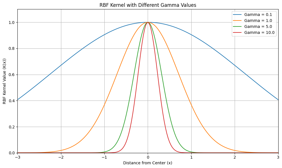
• Kernel Parameter (e.g., \(\gamma\) for RBF kernel): If using a kernel like RBF, there’s a kernel-specific parameter (gamma, \(\gamma\), for RBF kernel). \(\gamma\) controls the “width” or “influence” of each data point in defining the boundary.
  • Small \(\gamma\): Wider influence, smoother boundary, might lead to underfitting (boundary too loose, might miss some outliers).
  • Large \(\gamma\): Narrower influence, more complex, wigglier boundary, might lead to overfitting (boundary too tight, might flag normal points as outliers).

## Plotting different gamma values
import numpy as np
import matplotlib.pyplot as plt

def rbf_kernel(x, gamma):
    """
    Calculates the Radial Basis Function (RBF) kernel value.

    Args:
        x:  Distance from the center point.
        gamma: Gamma parameter, controlling the width of the RBF.

    Returns:
        The RBF kernel value.
    """
    return np.exp(-gamma * x**2)

# Define the range of x values to plot
x_values = np.linspace(-3, 3, 200)  # Range from -3 to 3, 200 points

# Define different gamma values to experiment with
gamma_values = [0.1, 1.0, 5.0, 10.0]

# Create the plot
plt.figure(figsize=(10, 6)) # Adjust figure size if needed

for gamma in gamma_values:
    rbf_vals = rbf_kernel(x_values, gamma)
    plt.plot(x_values, rbf_vals, label=f'Gamma = {gamma}')

plt.title('RBF Kernel with Different Gamma Values')
plt.xlabel('Distance from Center (x)')
plt.ylabel('RBF Kernel Value (K(x))')
plt.legend()
plt.grid(True) # Add grid for better readability
plt.xlim([-3, 3]) # Set x-axis limits for better focus
plt.ylim([0, 1.1]) # Set y-axis limits to be from 0 to slightly above 1
plt.tight_layout() # Adjust layout to prevent labels from overlapping
plt.show()

Decision Function:

After training, the One-Class SVM learns a decision function (often called decision_function(X) in scikit-learn). For a new data point \(\mathbf{x}_{new}\), this function outputs a score.

• Positive Score (typically > 0): Indicates that \(\mathbf{x}_{new}\) is considered “normal” (inside the learned boundary).
• Negative Score (typically < 0): Indicates that \(\mathbf{x}_{new}\) is considered “anomalous” (outside the learned boundary).

The magnitude of the score reflects the “confidence” or “distance” from the boundary. Scores closer to zero are closer to the boundary, while scores further from zero (in either positive or negative direction) are further away from the boundary.

Example Intuition:

Imagine you want to enclose a group of points on a 2D plane with a curve. One-Class SVM with an RBF kernel tries to find a curve that encloses most of these points, allowing for a certain fraction of points to be outside (controlled by \(\nu\)). The kernel parameter \(\gamma\) controls how flexible and wiggly this curve can be. New points are then classified based on whether they fall inside or outside this learned curve.

Prerequisites and Preprocessing for One-Class SVM

Before using One-Class SVM, understanding the prerequisites and preprocessing steps is crucial for getting good results.

Prerequisites & Assumptions:

• “Normal” Data Availability: One-Class SVM is designed for scenarios where you have a dataset primarily consisting of “normal” data points. You need to be able to identify and collect a representative set of normal examples for training.
• Feature Representation: Data should be represented as numerical features (vectors). One-Class SVM works with feature vectors to define boundaries in a multi-dimensional space.
• Outliers are truly rare: The assumption is that outliers (anomalies) are genuinely rare events in your training data. While the \(\nu\) parameter allows for some outliers in the training data, if your training set is heavily contaminated with anomalies, One-Class SVM might learn to consider anomalies as “normal,” and its anomaly detection performance will suffer.
• Data Distribution and Kernel Choice: The performance of One-Class SVM depends on the underlying distribution of your normal data and the choice of kernel. RBF kernel is versatile but might not be optimal for all data distributions. Linear kernel might be suitable if “normal” data can be separated linearly from outliers.

Assumptions (Implicit):

• Data is stationary: Assumes that the distribution of “normal” data remains relatively consistent over time. If the definition of “normal” changes significantly, the trained One-Class SVM might become less effective and require retraining.

Testing Assumptions (Informally):

• Data Visualization: Visualize your “normal” data (if possible, scatter plots for 2D or 3D data, feature histograms for higher dimensions). Look for patterns or clusters in your normal data. One-Class SVM works best when “normal” data forms relatively cohesive groups in the feature space.
• Outlier Ratio Check: Estimate the proportion of potential outliers in your training data. If you suspect your “normal” training data is heavily contaminated with anomalies, One-Class SVM might not be the best choice, or you might need to clean your data first.
• Experiment with Kernels: Try different kernels (linear, RBF, polynomial) and kernel parameters (gamma for RBF) and evaluate performance (using metrics discussed later) to find a kernel that works well for your data. RBF is often a good starting point due to its flexibility.

Python Libraries:

For implementing One-Class SVM in Python, the primary library you’ll use is:

• scikit-learn (sklearn): Scikit-learn provides the OneClassSVM class in its svm module. It’s a well-optimized and easy-to-use implementation.
• NumPy: For numerical operations and handling data as arrays, which Scikit-learn uses extensively.
• pandas: For data manipulation and working with DataFrames, if your data is in tabular format.
• Matplotlib or Seaborn: For data visualization, which can be helpful for understanding your data and visualizing the decision boundary (in 2D) or anomaly scores.

Data Preprocessing for One-Class SVM

Data preprocessing is crucial for One-Class SVM to perform well. Here are key preprocessing steps:

• Feature Scaling (Normalization/Standardization):
  • Why it’s essential: One-Class SVM, like standard SVMs and many distance-based algorithms, is sensitive to feature scales. Features with larger ranges can dominate distance calculations and influence the shape of the learned boundary disproportionately. Scaling is almost always necessary.
  • Preprocessing techniques (Strongly recommended):
    • Standardization (Z-score normalization): Scales features to have a mean of 0 and standard deviation of 1. Formula: \(z = \frac{x - \mu}{\sigma}\). Generally the most recommended scaling method for SVMs, including One-Class SVM, and often works very well.
    • Min-Max Scaling (Normalization): Scales features to a specific range, typically [0, 1] or [-1, 1]. Formula: \(x_{scaled} = \frac{x - x_{min}}{x_{max} - x_{min}}\). Can be used, but standardization is often empirically preferred for SVMs.
  • Example: If you are using features like “Transaction Amount” (range $0-$10,000) and “Customer Age” (range 18-90) for fraud detection. “Transaction Amount” has a much larger scale. Without scaling, One-Class SVM might primarily focus on transaction amount, and age might be underweighted. Scaling ensures both features contribute more equitably to the decision boundary.
  • When can it be ignored? Almost never. Feature scaling is almost always beneficial for One-Class SVM and very strongly recommended. You should only skip scaling if you have a very specific reason to believe that feature scales are inherently meaningful and should not be adjusted, which is rare in practice.
• Handling Categorical Features:
  • Why it’s important: One-Class SVM works with numerical feature vectors. Categorical features must be converted into a numerical representation.
  • Preprocessing techniques (Necessary for categorical features):
    • One-Hot Encoding: Convert categorical features into binary vectors. For example, “Day of Week” (Monday, Tuesday, …, Sunday) becomes 7 binary features: “Is_Monday,” “Is_Tuesday,” …, “Is_Sunday.” Suitable for nominal (unordered) categorical features.
    • Label Encoding (Ordinal Encoding): Assign numerical labels to categories. Suitable for ordinal (ordered) categorical features (e.g., “Education Level”: “High School”, “Bachelor’s”, “Master’s” -> 1, 2, 3). Less common for nominal categorical features.
  • Example: For network intrusion detection, if you have a feature “Protocol” (TCP, UDP, ICMP), one-hot encode it.
  • When can it be ignored? Only if you have only numerical features to begin with. Failing to encode categorical features before using One-Class SVM will lead to incorrect results or errors.
• Handling Missing Values:
  • Why it’s important: One-Class SVM, like standard SVMs, generally does not handle missing values directly. Missing values can disrupt distance calculations and boundary learning.
  • Preprocessing techniques (Essential to address missing values):
    • Imputation: Fill in missing values with estimated values. Common methods:
      • Mean/Median Imputation: Replace missing values with the mean or median of the feature. Simple and often a good starting point for SVM preprocessing. Median imputation might be slightly more robust to outliers.
      • KNN Imputation: Use K-Nearest Neighbors to impute missing values based on similar data points. Potentially more accurate but computationally more expensive for large datasets.
      • Model-Based Imputation: Train a predictive model to estimate missing values. More complex but potentially most accurate.
    • Deletion (Listwise - remove rows): Remove data points (rows) that have missing values. Use cautiously, as it can lead to loss of data, especially if missingness is not random. Only consider deletion if missing values are very few (e.g., <1-2%) and appear to be randomly distributed.
  • Example: In financial transaction data, if “Customer Income” is sometimes missing, use median imputation to replace missing income values with the median income of other customers.
  • When can it be ignored? Virtually never for One-Class SVM. You must handle missing values. Imputation is generally preferred over deletion to preserve data, unless missing values are extremely rare and deletion is inconsequential.
• Outlier Handling (Less Critical for Training Data - but relevant for test/new data):
  • Why less critical for training data: One-Class SVM is designed to detect outliers (anomalies). The \(\nu\) parameter explicitly allows for some data points in the “normal” training set to be treated as outliers (training errors). Thus, presence of a few outliers in your normal training data might be tolerated and even part of what the model learns as the “boundary” of normality.
  • Preprocessing techniques (for test data or if you want to pre-clean training data):
    • Outlier Removal (Pre-cleaning training data - optional): If you strongly believe your “normal” training data is significantly contaminated with obvious errors or noise-related outliers, you could consider pre-cleaning them using outlier detection methods (IQR, Z-score based outlier removal) before training the One-Class SVM. However, be cautious not to remove genuine, though slightly unusual, normal data points. Generally, for One-Class SVM, rely more on the algorithm’s own outlier detection capability rather than aggressive pre-cleaning of training data.
    • Robust Scaling: Using robust scalers (like RobustScaler in scikit-learn) can reduce the influence of outliers on feature scaling, making the scaling process less affected by extreme values, which can be beneficial.

Implementation Example: One-Class SVM in Python

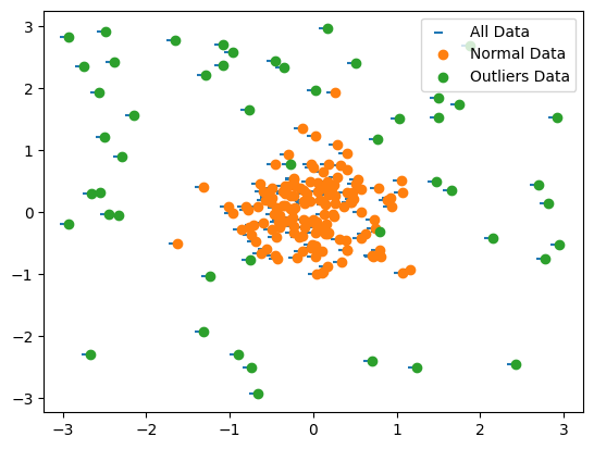
Let’s implement One-Class SVM using Python and scikit-learn. We’ll create dummy data with a clear “normal” cluster and some outliers.

Dummy Data:

We’ll generate synthetic data with a main cluster representing “normal” data and some scattered points as outliers.

## Loading libraries
import numpy as np
import pandas as pd
import matplotlib.pyplot as plt
from sklearn.model_selection import train_test_split
from sklearn.preprocessing import StandardScaler
from sklearn.svm import OneClassSVM

# Generate dummy "normal" data (cluster) and "anomalous" data (outliers)
np.random.seed(42)
normal_data = np.random.randn(150, 2) * 0.5 + [0, 0]  # Cluster around origin
outliers_data = np.random.uniform(low=-3, high=3, size=(50, 2)) # Scattered outliers
X = np.concatenate([normal_data, outliers_data]) # Combine
y = np.concatenate([np.ones(150), -np.ones(50)]) # 1 for normal, -1 for outlier (for evaluation, not used in training)
X_df = pd.DataFrame(X, columns=['feature_1', 'feature_2'])
y_series = pd.Series(y)

# Split data into training and testing sets (Crucial: train only on 'normal' data for OneClassSVM)
X_train = X_df[y_series == 1] # Training set is ONLY 'normal' data
X_test = X_df # Test set contains both 'normal' and 'anomalous' data
y_test = y_series # Test labels (for evaluation, not used in OneClassSVM training)

## Scatter plot of data points
plt.scatter(*zip(*X_df.to_numpy()),marker=0)
plt.scatter(*zip(*normal_data))
plt.scatter(*zip(*outliers_data))
plt.legend(["All Data", "Normal Data", "Outliers Data"])

# Scale the data using StandardScaler (important!)
scaler = StandardScaler()
X_train_scaled = scaler.fit_transform(X_train) # Fit scaler on TRAINING data ONLY
X_test_scaled = scaler.transform(X_test) # Apply scaler to TEST data

print("Dummy Training Data (first 5 rows of scaled normal features):")
print(pd.DataFrame(X_train_scaled, columns=X_train.columns).head())
print("\nDummy Test Data (first 5 rows of scaled features - includes normal and anomalous):")
print(pd.DataFrame(X_test_scaled, columns=X_test.columns).head())

Output:

    Dummy Training Data (first 5 rows of scaled normal features):
       feature_1  feature_2
    0   0.550082  -0.161377
    1   0.706548   1.501451
    2  -0.207371  -0.257338
    3   1.671957   0.745159
    4  -0.451252   0.520076
    
    Dummy Test Data (first 5 rows of scaled features - includes normal and anomalous):
       feature_1  feature_2
    0   0.550082  -0.161377
    1   0.706548   1.501451
    2  -0.207371  -0.257338
    3   1.671957   0.745159
    4  -0.451252   0.520076
    

# Initialize and fit OneClassSVM model
nu_value = 0.1 # nu parameter (fraction of outliers expected/allowed)
gamma_value = 'auto' # gamma parameter for RBF kernel ('scale' or 'auto' often good starting points, or float value)

oneclass_svm = OneClassSVM(kernel='rbf', nu=nu_value, gamma=gamma_value) # RBF kernel is common, tune kernel and nu/gamma
oneclass_svm.fit(X_train_scaled) # IMPORTANT: Fit ONLY on the scaled TRAINING data (normal data)

# Get predictions (1 for normal, -1 for outlier) on the TEST set
y_pred_test = oneclass_svm.predict(X_test_scaled)
X_test_labeled = X_test.copy()
X_test_labeled['prediction'] = y_pred_test # Add predictions to test DataFrame

# Get decision function values (raw scores, useful for thresholding and ranking anomalies)
decision_scores_test = oneclass_svm.decision_function(X_test_scaled)
X_test_labeled['decision_score'] = decision_scores_test # Add decision scores

print("\nPredictions (first 10):\n", y_pred_test[:10])
print("\nDecision Scores (first 10):\n", decision_scores_test[:10])

Output: Output (plot will be displayed, output will vary slightly):

(Output will show first 10 predictions (1 or -1) and decision scores. A contour plot will visualize the decision boundary learned by One-Class SVM, with regions classified as normal and outlier, and data points colored according to their predicted class.)

    
    Predictions (first 10):
     [ 1  1  1  1  1  1  1 -1  1  1]
    
    Decision Scores (first 10):
     [ 0.00118924  0.09482545  0.02152039  0.19006689  0.02197238  0.06130406
      0.02692327 -0.00024873  0.02203976  0.0191339 ]
    

# Visualize decision boundary and outliers (for 2D data)
xx, yy = np.meshgrid(np.linspace(-7, 7, 500), np.linspace(-7, 7, 500)) # Create grid for plotting boundary
Z = oneclass_svm.decision_function(np.c_[xx.ravel(), yy.ravel()]) # Get decision function values for grid
Z = Z.reshape(xx.shape)

plt.figure(figsize=(8, 6))
plt.contourf(xx, yy, Z, levels=np.linspace(Z.min(), 0, 7), cmap=plt.cm.Blues_r) # Contour for negative scores (outlier region)
a = plt.contour(xx, yy, Z, levels=[0], linewidths=2, colors='red') # Contour at 0 decision function (boundary)
plt.contourf(xx, yy, Z, levels=[0, Z.max()], colors='orange') # Contour for positive scores (normal region)

s = plt.scatter(X_train_scaled[:, 0], X_train_scaled[:, 1], color='white', s=20*4, edgecolors='k', label="Normal Training Data") # Normal training data (white)
b = plt.scatter(X_test_scaled[y_pred_test == -1, 0], X_test_scaled[y_pred_test == -1, 1], color='red', s=20*4, edgecolors='k', label="Predicted Outliers") # Predicted outliers (red)
c = plt.scatter(X_test_scaled[y_pred_test == 1, 0], X_test_scaled[y_pred_test == 1, 1], color='forestgreen', s=20*4, edgecolors='k', label="Predicted Normal") # Predicted normal (green)

plt.title('One-Class SVM: Decision Boundary and Outlier Detection')
plt.xlabel('Feature 1 (Scaled)')
plt.ylabel('Feature 2 (Scaled)')
plt.legend()
plt.grid(True)
plt.show()

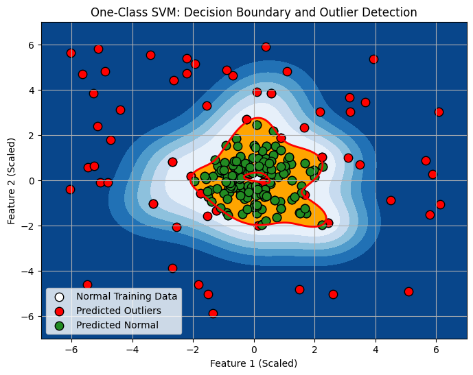
Explanation of Output:

• Predictions (first 10):: Shows the predictions for the first 10 data points in the test set. 1 indicates “normal,” and -1 indicates “outlier.” One-Class SVM aims to classify new data as either normal or outlier relative to the learned “normal” data distribution.
• Decision Scores (first 10):: Shows the decision function scores for the first 10 data points. Positive scores are on the “normal” side of the boundary, negative scores are on the “outlier” side. The magnitude of the score indicates the confidence of the classification.
• Plot: The visualization (if you run the plotting code) illustrates:
  • White points: The “normal” training data used to train the One-Class SVM.
  • Red points: Data points in the test set that are predicted as “outliers” (negative prediction).
  • Green points: Data points in the test set predicted as “normal” (positive prediction).
  • Red contour line: The decision boundary learned by One-Class SVM (where decision function is 0).
  • Blue filled region: Region with negative decision function values (outlier region).
  • Orange filled region: Region with positive decision function values (normal region).

Saving and Loading the Model and Scaler:

import pickle

# Save the scaler
with open('standard_scaler_oneclasssvm.pkl', 'wb') as f:
    pickle.dump(scaler, f)

# Save the OneClassSVM model
with open('oneclass_svm_model.pkl', 'wb') as f:
    pickle.dump(oneclass_svm, f)

print("\nScaler and One-Class SVM Model saved!")

# --- Later, to load ---

# Load the scaler
with open('standard_scaler_oneclasssvm.pkl', 'rb') as f:
    loaded_scaler = pickle.load(f)

# Load the OneClassSVM model
with open('oneclass_svm_model.pkl', 'rb') as f:
    loaded_oneclass_svm = pickle.load(f)

print("\nScaler and One-Class SVM Model loaded!")

# To use loaded model:
# 1. Preprocess new data using loaded_scaler
# 2. Use loaded_oneclass_svm.predict(new_scaled_data) to get outlier predictions for new data.
# 3. Use loaded_oneclass_svm.decision_function(new_scaled_data) to get decision scores.

This example provides a basic implementation and visualization of One-Class SVM for anomaly detection. You can experiment with different kernels, parameters (\(\nu\), \(\gamma\)), and datasets to further explore its capabilities.

Post-Processing: Thresholding and Anomaly Interpretation

After training a One-Class SVM, post-processing steps are important for interpreting the results and making practical use of the anomaly detection output.

1. Decision Score Thresholding:

• Purpose: Convert the continuous decision scores from decision_function() into binary anomaly classifications (normal/anomalous). You need to set a threshold value. Scores below the threshold are considered outliers.
• Methods for Setting Threshold:
  • Zero Threshold (Default for OneClassSVM): By default, in scikit-learn’s OneClassSVM, predictions are already binary (-1 for outlier, 1 for normal) based on a zero threshold on the decision function. If decision_function(X) < 0, it’s predicted as an outlier. You can use 0 as a threshold directly.

  • Percentile-Based Threshold: Calculate the decision scores on your normal training data. Find a percentile (e.g., 5th percentile) of these scores. Set this percentile value as your threshold. New data points with decision scores below this threshold are classified as anomalies. This approach is data-driven and tries to capture a certain percentage of training data as “inliers.”

  • Example (Percentile-Based Thresholding):

# Calculate decision scores on training data (normal data)
decision_scores_train = oneclass_svm.decision_function(X_train_scaled)

# Set threshold based on a percentile of training data scores (e.g., 5th percentile)
threshold_percentile = 5
threshold_value = np.percentile(decision_scores_train, threshold_percentile)

print(f"Decision Score Threshold (based on {threshold_percentile}th percentile of training data): {threshold_value:.4f}")

# Apply threshold to test data decision scores
y_pred_thresholded = np.where(decision_scores_test <= threshold_value, -1, 1) # -1 if score <= threshold, else 1

print("\nThresholded Predictions (first 10):\n", y_pred_thresholded[:10])

Output:

Decision Score Threshold (based on 5th percentile of training data): -0.0102

Thresholded Predictions (first 10):
 [1 1 1 1 1 1 1 1 1 1]

• Choosing the Threshold: The choice of threshold depends on the desired trade-off between false positives (normal data incorrectly flagged as anomaly) and false negatives (anomalies missed). A lower threshold will flag more points as anomalies (higher recall, lower precision for anomaly detection), and a higher threshold will flag fewer points (lower recall, higher precision for anomaly detection). You can adjust the threshold based on your application’s needs and the cost of false positives vs. false negatives.

2. Ranking Anomalies by Decision Score:

• Purpose: Instead of just binary classifications, use the decision scores themselves to rank data points by their “anomalousness.” Points with more negative decision scores are considered more anomalous.
• Technique: Use the raw decision scores directly as anomaly scores. Sort data points based on their decision scores in ascending order (most negative scores first). The most anomalous points will be at the top of the sorted list.
• Benefit: Ranking provides a more nuanced view of anomalousness than just binary labels and allows for prioritizing investigation of the most suspicious cases.
• Example (Ranking Anomalies):

# Get decision scores (already calculated as decision_scores_test)

# Create DataFrame with test data and decision scores for ranking
anomaly_ranking_df = X_test.copy()
anomaly_ranking_df['decision_score'] = decision_scores_test
anomaly_ranking_df = anomaly_ranking_df.sort_values(by='decision_score') # Sort by decision score (ascending)

print("\nAnomaly Ranking (Data points sorted by decision score, most anomalous first):\n")
print(anomaly_ranking_df.head(10)) # Show top 10 most anomalous

Output:

Anomaly Ranking (Data points sorted by decision score, most anomalous first):

     feature_1  feature_2  decision_score
192  -2.927073   2.819273       -2.297382
177  -2.490974   2.919837       -2.297382
193  -2.741041   2.346859       -2.297376
157  -2.381257   2.415317       -2.297351
180   2.916006   1.520269       -2.297271
186  -2.662180  -2.287093       -2.297205
191  -1.658425   2.779335       -2.297151
160  -0.664790  -2.934974       -2.297098
175  -2.563422   1.931160       -2.297038
161   2.432292  -2.452280       -2.296871

3. Feature Importance Analysis (Indirect, Less Direct than some Models):

• Purpose: Understand which features are most influential in determining anomaly scores. One-Class SVM doesn’t directly provide feature importance scores like some models (e.g., tree-based models or linear models with coefficients). However, you can infer feature importance indirectly.
• Techniques:
  • Sensitivity Analysis (Feature Perturbation): For each feature, perturb (slightly change) its values and observe how it affects the decision scores for data points. Features that, when perturbed, cause the largest changes in decision scores might be considered more influential.
  • Feature Ablation (Feature Removal): Train One-Class SVM models using subsets of features (leave-one-out feature sets). Compare the performance (e.g., anomaly detection metrics) of models trained with different feature subsets. Features whose removal leads to the greatest drop in performance could be considered more important.

4. Domain Knowledge Validation:

• Purpose: Validate the identified anomalies from a domain perspective. Do the flagged outliers make sense in the context of your problem? Are they genuinely unusual or suspicious?
• Action: Review the top-ranked anomalies (based on decision scores) with domain experts. See if they can provide insights into why these points were flagged and if they are indeed valid anomalies or potential errors. Domain expert validation is crucial for building trust in anomaly detection systems.

Post-processing steps are essential for turning the raw output of One-Class SVM into actionable insights and for building confidence in the anomaly detection results. Thresholding, ranking, feature importance analysis, and domain expert validation are all important components of a practical anomaly detection workflow using One-Class SVM.

Hyperparameter Tuning for One-Class SVM

The key hyperparameters to tune in One-Class SVM are:

• kernel: Specifies the kernel type. Common options are: 'linear', 'rbf', 'poly', 'sigmoid'.
  • kernel='linear': Simplest, creates a linear boundary. Fastest to train. Suitable if “normal” data is linearly separable from outliers.
  • kernel='rbf' (Radial Basis Function/Gaussian Kernel): Most versatile, creates non-linear boundaries, often curved or blob-like. Good default choice. Tuning gamma is crucial for RBF kernel.
  • kernel='poly' (Polynomial Kernel): Creates polynomial boundaries. Can capture curved relationships but might be more sensitive to parameter tuning. Tune degree and gamma.
  • kernel='sigmoid' (Sigmoid Kernel): Less frequently used for One-Class SVM compared to RBF or linear, but available. Tune gamma and coef0.
• nu (nu): Controls the trade-off between training errors (outliers in training data) and support vectors.
  • nu (range: (0, 1]):
    • Smaller nu (closer to 0): More strict outlier detection. Learns a tighter boundary around normal data. Might classify more normal points as outliers (increase false positives, decrease false negatives for anomalies). Fewer support vectors.
    • Larger nu (closer to 1): More lenient outlier detection. Learns a looser boundary, allowing more points to be considered “normal.” Might miss more true anomalies (decrease false positives, increase false negatives). More support vectors.
  • Tuning: Choose nu based on your application’s tolerance for false positives vs. false negatives. Experiment with values in the range [0.01, 0.1, 0.2, …, 0.5] or use grid search or cross-validation to find a good value.
• gamma (kernel coefficient): Parameter specific to kernels like 'rbf', 'poly', 'sigmoid'. Controls the influence of individual training samples.
  • gamma='scale' (default for RBF in scikit-learn > 0.22): Gamma is set to 1 / (n_features * X.var()). Data-dependent scaling. Often a good starting point.
  • gamma='auto' (alternative): Gamma is set to 1 / n_features. Another data-dependent heuristic.
  • gamma (float value): You can set a specific float value for gamma.
    • Smaller gamma: Wider kernel influence, smoother decision boundary, can lead to underfitting.
    • Larger gamma: Narrower kernel influence, wigglier decision boundary, can lead to overfitting (boundary too sensitive to training data, might not generalize well).
  • Tuning: For RBF kernel, tuning gamma is critical. Experiment with values in a logarithmic scale (e.g., [0.001, 0.01, 0.1, 1, 10, 100]) or use techniques like grid search or cross-validation to find a good value that balances bias and variance.
• degree (for kernel='poly'): Degree of the polynomial kernel function.
  • Effect: Higher degree allows for more complex, higher-order polynomial boundaries.
  • Tuning: If using polynomial kernel, tune degree (e.g., try 2, 3, 4). Higher degrees increase model complexity and computational cost.
• coef0 (for kernel='poly' and kernel='sigmoid'): Independent term in polynomial and sigmoid kernels.
  • Effect: Shifts the decision boundary. Can sometimes help in fine-tuning, but less commonly tuned than gamma or nu.
  • Tuning: If using polynomial or sigmoid kernel, you could experiment with coef0 values, but often leave it at its default (0.0).

Hyperparameter Tuning Methods:

• Manual Tuning and Visualization (for 2D data, understanding parameters): Experiment with different values of kernel, nu, gamma (and degree if using polynomial). Visualize the decision boundary (for 2D data) and visually assess if the boundary seems to appropriately enclose the normal data and separate outliers. Useful for gaining intuition about parameter effects.
• Grid Search with Evaluation Metric: Use grid search combined with a suitable evaluation metric to automate hyperparameter selection. For anomaly detection evaluation, you might use metrics like:
  • Precision, Recall, F1-score (treating anomalies as “positive” class): If you have labeled data (even if only for evaluation, not training). Optimize for F1-score to balance precision and recall.
  • AUC (Area Under ROC Curve): If you have anomaly labels and want to optimize the trade-off between true positive rate and false positive rate across different thresholds.
  • Note: For true One-Class SVM in unsupervised settings (where you only have “normal” training data and no labels during training), cross-validation might be less directly applicable in the traditional supervised sense. You might use cross-validation on your normal training data itself and evaluate on a separate labeled test set to assess generalization performance on anomaly detection.

Example: Grid Search for Hyperparameter Tuning (using GridSearchCV and F1-score for illustration, assuming you have some labeled data for evaluation, though One-Class SVM is primarily unsupervised).

from sklearn.model_selection import GridSearchCV
from sklearn.metrics import f1_score, make_scorer

# Define parameter grid to search
param_grid = {
    'kernel': ['rbf'], # Or ['linear', 'rbf', 'poly']
    'nu': [0.001, 0.01, 0.05, 0.1, 0.2], # Example nu values
    'gamma': ['scale', 'auto', 0.0001, 0.01, 0.03, 0.05, 0.1, 0.5, 1, 10] # Example gamma values
}

# Define a scorer (e.g., F1-score, assuming you have anomaly labels in y_test, treat anomalies as positive class - label -1)
anomaly_f1_scorer = make_scorer(f1_score, average='binary', pos_label=-1, zero_division=1) # Anomalies are labeled -1

# Initialize GridSearchCV with OneClassSVM and parameter grid
grid_search = GridSearchCV(OneClassSVM(), param_grid, scoring=anomaly_f1_scorer, cv=3) # 3-fold cross-validation

# Fit GridSearchCV on the training data (scaled normal data)
grid_search.fit(X_train_scaled, y_series[y_series == 1]) # y_series[y_series == 1] - dummy labels, OneClassSVM ignores y in fit

# Get the best model and best parameters from GridSearchCV
best_ocsvm = grid_search.best_estimator_
best_params = grid_search.best_params_
best_score = grid_search.best_score_

print("\nBest One-Class SVM Model from Grid Search:")
print(best_ocsvm)
print("\nBest Hyperparameters:", best_params)
print(f"Best Cross-Validation F1-Score: {best_score:.4f}")

# Evaluate best model on the test set
y_pred_best = best_ocsvm.predict(X_test_scaled)
f1_test_best = f1_score(y_test, y_pred_best, pos_label=-1) # Evaluate on test set using F1-score
print(f"F1-Score on Test Set (Best Model): {f1_test_best:.4f}")

Output:

Best One-Class SVM Model from Grid Search:
OneClassSVM(gamma=0.0001, nu=0.01)

Best Hyperparameters: {'gamma': 0.0001, 'kernel': 'rbf', 'nu': 0.01}
Best Cross-Validation F1-Score: 0.6667
F1-Score on Test Set (Best Model): 0.9149

Important Note for Hyperparameter Tuning with One-Class SVM:

• Unsupervised Nature: One-Class SVM is primarily an unsupervised anomaly detection method. You train it only on “normal” data. Traditional cross-validation for hyperparameter tuning is less directly applicable in a purely unsupervised setting. Grid search combined with evaluation metrics (like Silhouette score or anomaly detection metrics if labeled validation data is available) is often used.
• Validation Approach: For hyperparameter tuning, consider:
  1. Using a labeled validation set (if available): Split your labeled data into training (normal only), validation (normal + anomalies), and test (normal + anomalies). Train One-Class SVM on training data, tune hyperparameters using validation set and anomaly detection metrics, and finally evaluate on the test set.
  2. Using internal validation metrics on normal data: If no labeled validation data, you could try using metrics like Silhouette score on your normal training data itself (though this might be less reliable for anomaly detection than metrics that directly evaluate anomaly separation).

Checking Model Accuracy: Anomaly Detection Metrics

“Accuracy” in the context of One-Class SVM for anomaly detection needs to be evaluated using metrics appropriate for anomaly detection tasks, not just classification accuracy in the standard sense. Since anomaly detection is often framed as identifying a minority class (anomalies), metrics need to reflect the performance in detecting these rare events.

Relevant Anomaly Detection Metrics (assuming you have some labeled data for evaluation, even though One-Class SVM is primarily unsupervised):

• Precision, Recall, F1-score (for Anomaly Class): Treat “anomaly” as the “positive” class.
  • Precision (for anomalies): Out of all points predicted as anomalies, what fraction are truly anomalies? (Minimize false positives - normal points incorrectly flagged as anomalies). Formula: \(Precision_{anomaly} = \frac{True\ Positives (TP)}{True\ Positives (TP) + False\ Positives (FP)}\), where TP and FP are with respect to anomaly class.
  • Recall (for anomalies): Out of all actual anomalies, what fraction were correctly detected by the model? (Minimize false negatives - anomalies missed and classified as normal). Formula: \(Recall_{anomaly} = \frac{True\ Positives (TP)}{True\ Positives (TP) + False\ Negatives (FN)}\), where TP and FN are with respect to anomaly class.
  • F1-score (for anomalies): Harmonic mean of precision and recall. Provides a balanced measure. Formula: \(F1-score_{anomaly} = 2 \times \frac{Precision_{anomaly} \times Recall_{anomaly}}{Precision_{anomaly} + Recall_{anomaly}}\).
  • Use case: When you have labeled data (even if only for evaluation) and want to assess the balance between correctly identifying anomalies and minimizing false alarms. F1-score is a good overall metric when you want to balance precision and recall.
• AUC (Area Under the ROC Curve): (Area Under Receiver Operating Characteristic Curve). Measures the ability of the model to distinguish between normal and anomalous points at various threshold settings.
  • ROC Curve: Plots True Positive Rate (Recall for anomalies) vs. False Positive Rate (False Alarm Rate - normal points classified as anomalies) at different decision thresholds.
  • AUC Score: Area under the ROC curve. Ranges from 0 to 1. AUC of 0.5 is no better than random guessing, AUC of 1 is perfect classification. Higher AUC is better for anomaly detection.
  • Use case: When you want to evaluate the model’s ability to rank anomalies effectively and are interested in the trade-off between true positive rate and false positive rate. AUC is less sensitive to class imbalance than accuracy.
• Accuracy (Overall, but less informative for anomaly detection): Overall accuracy (percentage of correct classifications for both normal and anomaly classes). Can be misleading if anomaly class is very rare (imbalanced data). In anomaly detection, you are often more concerned with performance specifically on the anomaly class (precision, recall, F1-score for anomalies, AUC) than overall accuracy.

Calculating Metrics in Python (using scikit-learn metrics):

from sklearn.metrics import precision_score, recall_score, f1_score, roc_auc_score

# --- Assume you have y_test (true labels, 1 for normal, -1 for anomaly) and y_pred_test (OneClassSVM predictions) ---

# Calculate Precision, Recall, F1-score for anomaly class (label -1)
precision_anomaly = precision_score(y_test, y_pred_test, pos_label=-1)
recall_anomaly = recall_score(y_test, y_pred_test, pos_label=-1)
f1_anomaly = f1_score(y_test, y_pred_test, pos_label=-1)

print("\nAnomaly Detection Metrics (Anomaly class = -1):")
print(f"Precision (Anomalies): {precision_anomaly:.4f}")
print(f"Recall (Anomalies): {recall_anomaly:.4f}")
print(f"F1-Score (Anomalies): {f1_anomaly:.4f}")

# Calculate AUC (requires probability scores, OneClassSVM decision_function can be used as score)
auc_score = roc_auc_score(y_test == -1, decision_scores_test) # y_test == -1 makes anomaly class 'True' for AUC calculation
print(f"AUC Score: {auc_score:.4f}")

# Overall Accuracy (less emphasized for anomaly detection, but for completeness)
from sklearn.metrics import accuracy_score
overall_accuracy = accuracy_score(y_test, y_pred_test)
print(f"Overall Accuracy: {overall_accuracy:.4f}")

Output:

Anomaly Detection Metrics (Anomaly class = -1):
Precision (Anomalies): 0.7778
Recall (Anomalies): 0.9800
F1-Score (Anomalies): 0.8673
AUC Score: 0.0199
Overall Accuracy: 0.9250

Interpreting Metrics:

• Higher Precision, Recall, F1-score (for anomalies) are better. Choose metrics and threshold based on your application’s priorities (e.g., prioritize high recall if missing anomalies is very costly, prioritize high precision if false alarms are very costly).
• Higher AUC is better. AUC provides an overall measure of how well the model can discriminate between normal and anomalous data across different thresholds.
• Context Matters: Interpret metric values in the context of your specific problem and the expected rarity of anomalies. For highly imbalanced datasets (very few anomalies), even seemingly “good” accuracy might not be sufficient if anomaly detection metrics (precision, recall, F1, AUC for anomalies) are poor. Focus on anomaly-specific metrics in anomaly detection tasks.

Model Productionizing Steps for One-Class SVM

Productionizing a One-Class SVM model for anomaly detection involves deploying it to monitor new data and flag anomalies in a real-world setting.

1. Save the Trained Model and Preprocessing Objects:

As shown in the implementation example, save:

• Scaler: The fitted scaler (e.g., StandardScaler).
• OneClassSVM Model: The trained OneClassSVM model object.

2. Create an Anomaly Detection Service/API:

• Purpose: To make your One-Class SVM model accessible for real-time anomaly detection on new incoming data.
• Technology Choices (Similar to other models): Python frameworks (Flask, FastAPI), web servers, cloud platforms, Docker for containerization (see previous blog posts).
• API Endpoints (Example using Flask):
  • /detect_anomaly: Endpoint to take new data as input and return anomaly predictions (normal/anomalous classification).
  • /anomaly_score: Endpoint to return the decision function score (raw anomaly score) for input data, allowing for thresholding and ranking on the client side.
• Example Flask API Snippet (for anomaly detection):

from flask import Flask, request, jsonify
import pandas as pd
import pickle

app = Flask(__name__)

# Load OneClassSVM model and scaler
oneclass_svm_model = pickle.load(open('oneclass_svm_model.pkl', 'rb'))
data_scaler = pickle.load(open('standard_scaler_oneclasssvm.pkl', 'rb'))

@app.route('/detect_anomaly', methods=['POST'])
def detect_anomaly():
    try:
        data_json = request.get_json()
        if not data_json:
            return jsonify({'error': 'No JSON data provided'}), 400

        input_df = pd.DataFrame([data_json]) # Input data as DataFrame
        input_scaled = data_scaler.transform(input_df) # Scale input data
        prediction = oneclass_svm_model.predict(input_scaled).tolist() # Get prediction

        return jsonify({'prediction': prediction[0]}) # Return single prediction

    except Exception as e:
        return jsonify({'error': str(e)}), 500

if __name__ == '__main__':
    app.run(debug=True) # debug=True for local testing, remove for production

3. Deployment Environments (Same as discussed in previous blogs):

• Local Testing: Flask app locally.
• On-Premise Deployment: Deploy on your organization’s servers.
• Cloud Deployment (PaaS, Containers, Serverless): Cloud platforms (AWS, Google Cloud, Azure) for scalable API deployment. Serverless functions can be very cost-effective for anomaly detection services that are not constantly under heavy load.

4. Monitoring and Maintenance (Focus on Data Drift and Threshold Adjustment):

• Monitoring Data Drift: Crucial for anomaly detection. Monitor the distribution of incoming data over time. If the distribution of “normal” data starts to drift significantly, the trained One-Class SVM model might become less accurate and need retraining.
• Performance Monitoring: Track API performance metrics (latency, error rates). Monitor anomaly detection performance metrics if you have ground truth labels for incoming data (e.g., precision, recall, false positive rate).
• Threshold Adjustment: The optimal threshold for anomaly detection might need adjustment over time based on real-world performance and changing data distributions. You might need to periodically re-evaluate and adjust the decision threshold.
• Model Retraining: Retrain your One-Class SVM model periodically with updated “normal” data to adapt to concept drift and maintain anomaly detection effectiveness.

5. Real-time vs. Batch Anomaly Detection:

• Real-time: Deploy the API for real-time anomaly detection if you need to flag anomalies immediately as new data arrives (e.g., for fraud detection, network intrusion detection).
• Batch: For batch anomaly detection (e.g., nightly analysis of manufacturing data, monthly review of transaction logs), you can run your One-Class SVM prediction scripts in a batch processing pipeline (using cloud batch services or scheduled jobs) to process data and generate anomaly reports.

Productionizing One-Class SVM for anomaly detection requires careful attention to data preprocessing, model deployment, continuous monitoring for data drift, and threshold management to ensure the system remains accurate and effective over time.

Conclusion: One-Class SVM - A Powerful Tool for Spotting the Unexpected

One-Class SVM is a valuable and versatile algorithm for anomaly detection, particularly effective when you primarily have access to “normal” data and need to identify deviations from this normality. Its ability to learn complex, non-linear boundaries around data and its robustness through the kernel trick make it a strong tool in various applications.

Real-world Applications where One-Class SVM is particularly useful:

• Situations with Imbalanced Data: Anomaly detection problems are inherently imbalanced (anomalies are rare). One-Class SVM is designed to handle this imbalance by focusing on modeling only the normal class.
• Novelty Detection: Scenarios where you are looking for completely new types of anomalies that were not seen during training. One-Class SVM aims to define “normal” so that anything truly novel (outside this definition) can be flagged.
• Domains with Limited Anomaly Examples: Applications where collecting labeled anomaly data is difficult, expensive, or rare. You can train One-Class SVM effectively using only readily available “normal” data.
• High-Dimensional Data: SVMs, including One-Class SVM, can often handle high-dimensional data relatively well due to their focus on support vectors and kernel methods.
• Non-linear Anomaly Boundaries: When anomaly boundaries are not linear (e.g., anomalies might appear in clusters of unusual shapes), the RBF kernel in One-Class SVM provides the flexibility to learn non-linear, complex boundaries.

Optimized or Newer Algorithms and Alternatives:

While One-Class SVM is a powerful anomaly detection method, there are other algorithms and approaches, some of which might be more suitable depending on the specific characteristics of your data and problem:

• Isolation Forest: An ensemble method specifically designed for anomaly detection. Often faster than One-Class SVM, especially for high-dimensional data, and can be more interpretable.
• Local Outlier Factor (LOF): A density-based anomaly detection algorithm that identifies anomalies based on their local density compared to their neighbors. Effective in detecting local outliers.
• Autoencoders (Deep Learning): Neural network-based autoencoders can be trained on normal data. Anomalies are detected based on high reconstruction error when trying to reconstruct anomalous input data. Useful when you want to learn complex, non-linear representations of normality.
• Gaussian Mixture Models (GMMs): Probabilistic models that can represent normal data as a mixture of Gaussian distributions. Anomalies are points with low probability under the learned Gaussian mixture model.
• Robust Covariance Estimation (e.g., Elliptic Envelope in scikit-learn): Assumes normal data is multivariate Gaussian and uses robust covariance estimators to define an ellipsoidal boundary around normal data. Efficient for lower-dimensional data that is approximately Gaussian.

Conclusion:

One-Class SVM is a robust and versatile algorithm for anomaly detection, offering a powerful approach when you primarily have access to normal data. Understanding its principles, hyperparameters, preprocessing requirements, and evaluation metrics equips you to effectively apply it to various anomaly detection challenges in diverse real-world domains. Consider One-Class SVM alongside other anomaly detection techniques and choose the method that best aligns with your data characteristics, application needs, and desired balance between accuracy, interpretability, and computational efficiency.

References

1. Schölkopf, B., Platt, J. C., Shawe-Taylor, J., Smola, A. J., & Williamson, R. C. (2001). Estimating the support of a high-dimensional distribution. Neural computation, 13(7), 1443-1471. [Link to MIT Press Journals (may require subscription or institutional access)] - The seminal paper introducing the One-Class SVM algorithm.

2. Tax, D. M. J., & Duin, R. P. W. (2004). Support vector data description. Machine learning, 54(1), 45-66. [Link to SpringerLink (may require subscription or institutional access)] - Another important paper discussing Support Vector Data Description (SVDD), a closely related method to One-Class SVM, and its application to one-class classification.

3. Scikit-learn documentation on OneClassSVM: [Link to scikit-learn OneClassSVM documentation] - Official scikit-learn documentation, providing practical examples, API reference, and implementation details for the OneClassSVM class.

4. Hodge, V. J., & Austin, J. (2004). A survey of outlier detection methodologies. Artificial intelligence review, 22(2), 85-126. [Link to SpringerLink (may require subscription or institutional access)] - A comprehensive survey of various outlier detection techniques, providing context for One-Class SVM within the broader field of anomaly detection.

5. Chandola, V., Banerjee, A., & Kumar, V. (2009). Anomaly detection: A survey. ACM computing surveys (CSUR), 41(3), 1-58. [Link to ACM Digital Library (may require subscription)] - Another influential survey paper providing a broad overview of anomaly detection methods and applications, placing One-Class SVM in a wider perspective of anomaly detection approaches.

This blog post provides a detailed introduction to One-Class SVM for anomaly detection. Experiment with the provided code examples, tune hyperparameters, and apply it to your own datasets to gain practical experience and deeper understanding of this valuable anomaly detection algorithm.